Meta-Learning and Universality

Transcript

1 Meta-Learning and Universality Conference paper at ICLR 2018 Chelsea Finn & Sergey Levine (US Berkeley) Youngseok Yoon

2 Contents The Universality in Meta-Learning Model Construct (Pre-update) Single gradient step and Post-update Show universality from model Experiments Conclusion

3 The Universality in Meta-Learning What is the universality in Meta-Learning? Universality in Neural Network: Approximate any function ff: xx yy Universality in Meta-Learning: Approximate any function ff: xx, yy kk, xx yy Input: The training data xx, yy kk, and Test data xx. In this presentation, only show about kk = 1 case. Our model to verify Universality: MAML: ff ; θθ ff( ; θθ ), θθ = θθ αα θθ L tttttttttttt, ff ; θθ Update model ff( ; θθ) using gradient update

4 Model Construct (Pre-update) Our model: Deep neural network with ReLU, MAML training.

5 Model Construct (Pre-update) Construct model ff ; θθ with ReLU If we assume inputs and all pre-synaptic activations are nonnegative, then deep ReLU act like deep linear networks. (1) ff ; θθ = ff oooooo NN ii=1 WW ii φφ ; θθ ffff, θθ bb ; θθ oooooo

6 Single gradient step and Post-update WWii L = aa ii bb ii 1 aa ii : the error gradient with respect to the pre-synaptic activations at layer ii bb ii 1 : the forward post-synaptic activations at layer ii 1 ffffffffffffff WW ii+1 bb ii 1 WW ii aa ii WW ii 1

7 Single gradient step and Post-update let zz = Then, NN ii=1 WW ii φφ xx; θθ ffff, θθ bb, zz L = ee(xx, yy) WWii L = aa ii bb ii 1 = WW ii 1 WW NN 1 ee xx, yy jj=ii+1 WW jj φφ xx; θθ ffff, θθ bb = ii 1 jj=1 WW jj ee xx, yy φφ xx; NN θθffff, θθ bb jj=ii+1 WW jj ffffffffffffff WW ii+1 bb ii 1 WW ii aa ii WW ii 1

8 Single gradient step and Post-update let zz = Then, NN ii=1 WW ii φφ xx; θθ ffff, θθ bb, zz L = ee(xx, yy) WWii L = aa ii bb ii 1 = WW ii 1 WW NN 1 ee xx, yy jj=ii+1 WW jj φφ xx; θθ ffff, θθ bb = ii 1 jj=1 WW jj ee xx, yy φφ xx; NN θθffff, θθ bb jj=ii+1 WW jj Therefore, post-update value of NN ii=1 NN ii=1 NN WW ii αασ ii=1 ii 1 jj=1 WW jj WW NN ii = ii=1 ii 1 WW jj ee xx, yy φφ xx; θθffff, θθ bb jj=ii+1 NN jj=1 WW ii αα WWii L WW ii 1 jj jj=1 WW jj OO αα 2

9 Single gradient step and Post-update Post-update value of NN ii=1 NN ii=1 NN WW ii αασ ii=1 ii 1 jj=1 WW jj jj=1 WW NN ii = ii=1 WW ii αα WWii L ii 1 WW jj ee xx, yy φφ xx; θθffff, θθ bb jj=ii+1 NN WW ii 1 jj jj=1 WW jj OO αα 2 Now, post-update value of zz when xx input into ff ; θθ NN zz = ii=1 WW ii φφ xx ; θθ ffff, θθ bb = NN ii=1 WW ii φφ xx ; θθ ffff, θθ bb NN ii 1 WW jj ee xx, yy φφ xx; NN θθffff, θθ bb jj=ii+1 αασ ii=1 ii 1 jj=1 WW jj And, ff xx ; θθ jj=1 = ff oooooo zz ; θθ oooooo WW ii 1 jj jj=1 WW jj φφ xx ; θθ ffff, θθ bb

10 Show universality from model How to show universality from post-updated model?

11 Show universality from model Use independently control information flow from xx, from yy, from xx by multiplexing forward information from xx and backward information from yy Decomposing WW ii, φφ and error gradient into three parts, WW ii WW ii WW ii 0, φφ ; θθ ffff, θθ bb 0 0 ww ii φφ ; θθ ffff, θθ bb 00, zz L yy, ff xx; θθ θθ bb 00 ee yy ee yy 2

12 Show universality from model xx θθ ffff, θθ bb WW NN WW ii WW 1 zz ff oooooo yy xx θθ ffff, θθ bb φφ 00 θθ bb WW NN WW NN ww NN WW ii WW ii ww ii WW 1 WW 1 ww 1 zz zz zz ff oooooo yy

13 Show universality from model Then, before the gradient update, zz = zz zz zz = NN WW ii φφ(xx; θθ ffff, θθ bb ) ii= Hence, represent the middle one of after gradient update, zz zz = NN ii=1 φφ xx; θθ ffff, θθ bb 00 θθ bb WW ii WW ii ww ii NN jj=ii+1 φφ xx; θθ ffff, θθ bb 00 θθ bb WW jj WW jj ww jj NN αασ ii=1 ii 1 jj=1 ii 1 jj=1 WW jj 0 0 ii 1 0 WW jj 0 jj=1 0 0 ww jj WW jj 0 0 φφ xx ; θθ ffff, θθ bb 0 WW jj ww jj θθ bb WW jj WW jj ww jj 00 ee yy ee yy zz NN = αασ ii=1 ii 1 jj=1 WW jj ii 1 jj=1 WW jj ee yy φφ xx; θθ ffff, θθ bb jj=ii+1 NN ii 1 WW jj jj=1 WW jj φφ xx ; θθ ffff, θθ bb

14 Show universality from model yy = ff oooooo zz; θθ oooooo and zz = 0 xx θθ ffff, θθ bb φφ 00 θθ bb WW NN WW NN ww NN WW ii WW ii ww ii WW 1 WW 1 ww 1 zz zz zz ff oooooo yy zz NN = αασ ii=1 ii 1 jj=1 WW jj ii 1 jj=1 WW jj ee yy φφ xx; θθ ffff, θθ bb jj=ii+1 = αασ NN ii=1 AA ii ee yy φφ xx; θθ ffff, θθ bb BBii BB ii φφ xx ; θθ ffff, θθ bb (3) NN ii 1 WW jj jj=1 WW jj φφ xx ; θθ ffff, θθ bb xx θθ ffff, θθ bb φφ 00 θθ bb WW NN WW NN ww NN WW ii WW ii ww ii WW 1 WW 1 ww 1 zz zz zz ff oooooo yy

15 Show universality from model Path 1) Define ff oooooo Path 2) Show zz as new vector vv, which containing informations of xx, yy and xx At last, Universality with Vector vv

16 Show universality from model Define ff oooooo as a neural network that approximates the following multiplexer function and its derivatives ff oooooo zz zz zz zz ; θθ oooooo = 11 zz=0 gg pppppp ; θθ gg + 11 zz 0 h pppppppp zz; θθ h, 4 zz zz Where gg pppppp is a linear function with parameters θθ gg such that zz L = ee yy (2) Where h pppppppp is a neural network with one or more hidden layers. Then, after pose-update, ff oooooo zz zz zz ; θθ oooooo = h pppppppp zz ; θθ h, 5 xx θθ ffff, θθ bb φφ 00 θθ bb WW NN WW NN ww NN WW ii WW ii ww ii WW 1 WW 1 ww 1 zz zz zz gg pppppp h pppppppp yy

17 Show universality from model Change the form of zz with kernel form zz = αασ NN ii=1 AA ii ee yy φφ xx; θθ ffff, θθ bb BBii BB ii φφ xx ; θθ ffff, θθ bb = NN αασii=1 AA ii ee yy kk ii xx, xx zz = αασ NN ii=1 AA ii ee yy kk ii xx, xx has the all information of xx, yy and xx. Assume ee yy is a linear function of yy which can extract the original information yy. xx θθ ffff, θθ bb φφ 00 θθ bb WW NN WW NN ww NN WW ii WW ii ww ii WW 1 WW 1 ww 1 zz zz zz gg pppppp h pppppppp yy

18 Show universality from model Change the form of zz with kernel form zz = αασ NN ii=1 AA ii ee yy φφ xx; θθ ffff, θθ bb BBii BB ii φφ xx ; θθ ffff, θθ bb = NN αασii=1 AA ii ee yy kk ii xx, xx zz = αασ NN ii=1 AA ii ee yy kk ii xx, xx has the all information of xx, yy and xx. Assume ee yy is a linear function of yy which can extract the original information yy. Idea 1) Decompose index ii = 1,, NN to a product of jj = 0,, JJ 1 aaaaaa ll = 0,, LL 1, and then assign those to xx aaaaaa xx Idea 2) Discretize xx and xx to jj and ll by kernel kk(, ) Idea 3) Make new vector vv, which contain all information of xx, xx aaaaaa yy from AA ii, ee yy aaaaaa kk ii

19 Show universality from model Idea 1) Decompose index ii = 1,, NN to a product of jj = 0,, JJ 1 aaaaaa ll = 0,, LL 1, and then assign those to xx aaaaaa xx zz = αασ NN ii=1 AA ii ee yy kk ii xx, xx = αασ JJ 1 jj=0 Σ ll=0 LL 1 AA jjjj Idea 2) Discretize xx and xx to jj and ll by kernel kk(, ) kk jjjj xx, xx = 1 0 iiii dddddddddd xx = ee jj aaaaaa dddddddddd xx ooooooooooooooooo ee yy kk jjjj xx, xx = ee ll (6) xx θθ ffff, θθ bb φφ 00 θθ bb WW NN WW NN ww NN WW ii WW ii ww ii WW 1 WW 1 ww 1 zz zz zz gg pppppp h pppppppp yy

20 Show universality from model Idea 3) Make new vector vv, which contain all information of xx, xx aaaaaa yy from AA ii, ee yy aaaaaa kk ii Choose ee yy to be a linear function that outputs J LL stacked copies of yy εε εε Define AA jjjj to be a select yy at the position of (jj, ll) = jj + JJ LL, AA jjjj = 1 + εε, 1 + εε at position (jj, ll) εε εε As a result, zz = αασ NN ii=1 AA ii ee yy kk ii xx, xx 0 0 = vv xx, xx, yy yy 0 0 xx = αασ JJ 1 jj=0 Σ ll=0 θθ ffff, θθ bb LL 1 AA jjjj φφ 00 θθ bb ee yy kk jjjj xx, xx WW NN WW NN ww NN WW ii WW ii ww ii WW 1 WW 1 ww 1 zz zz zz gg pppppp h pppppppp yy

21 Show universality from model As a result, zz = αασ NN ii=1 AA ii ee yy kk ii xx, xx ff xx ; θθ = αασ JJ 1 jj=0 Σ ll=0 h pppppppp αααα xx, xx, yy ; θθ h LL 1 AA jjjj ee yy kk jjjj xx, xx = αααα xx, xx, yy, where vv xx, xx, yy It is a universal function approximator with respect to its inputs xx, xx, yy 0 0 yy 0 0 xx θθ ffff, θθ bb φφ 00 θθ bb WW NN WW NN ww NN WW ii WW ii ww ii WW 1 WW 1 ww 1 zz zz zz gg pppppp h pppppppp yy

22 Experiments Q1) Is there empirical benefit to using one meta-learning approach versus another, and in which case? A1) Empirically show the inductive bias of gradient-based vs recurrent meta-learners Explore the differences between gradient-based vs recurrent A learner trained with MAML, improve or start to overfit after additional gradient steps. Better few-shot learning performance on tasks outside of the training distribution?

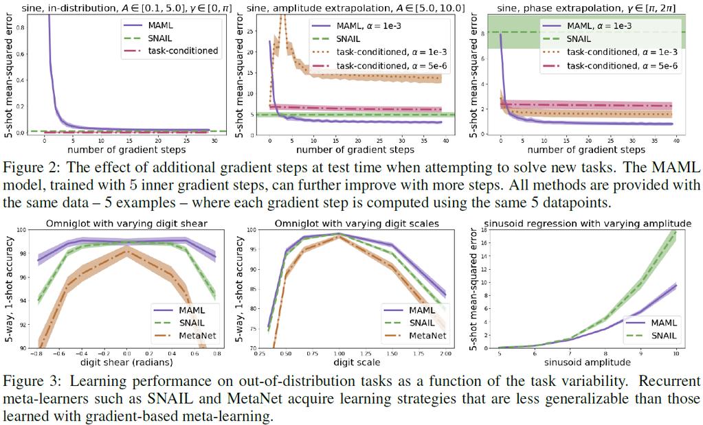
23 Experiments

24 Experiments

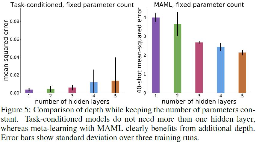
25 Experiments Q2) Theory suggest that deeper networks lead to increased expressive power for representing different learning procedures. Is it right? A1) Investigate the role of model depth in gradient-based metalearning

26 Experiments

27 Conclusion Meta-learners that use standard gradient descent with a sufficiently deep representation can approximate any learning procedure, and are equally expressive as recurrent learners. In experiments, MAML is more successful when faced with out-of-domain tasks compared to recurrent model We formalize what it means for a meta-learner to be able to approximate any learning algorithm in terms of its ability to represent functions of the dataset and test inputs.

28 Appendix A B C we assume inputs and all pre-synaptic activations are non-negative, then deep ReLU act like deep linear networks. (1) zz NN = αασ ii=1 ii 1 jj=1 WW jj ii 1 jj=1 WW jj ee yy φφ xx; θθ ffff, θθ bb jj=ii+1 = αασ NN ii=1 AA ii ee yy φφ xx; θθ ffff, θθ bb BBii BB ii φφ xx ; θθ ffff, θθ bb (3) zz L yy, ff xx; θθ ff oooooo zz zz zz kk jjjj xx, xx = ee yy ee yy 2 ; θθ oooooo = 11 zz=0 gg pppppp zz zz zz iiii dddddddddd xx = ee jj aaaaaa dddddddddd xx NN ii 1 WW jj jj=1 WW jj h zz; θθ, 4, ff ; θθ gg + 11 zz 0 zz zz pppppppp h oooooo zz ooooooooooooooooo = ee ll (6) φφ xx ; θθ ffff, θθ bb ; θθ oooooo = h pppppppp zz ; θθ h, 5

29 Appendix A zz NN = αασ ii=1 ii 1 jj=1 WW jj ii 1 jj=1 WW jj ee yy φφ xx; θθ ffff, θθ bb = αασ NN ii=1 AA ii ee yy φφ xx; θθ ffff, θθ bb BBii BB ii φφ xx ; θθ ffff, θθ bb Choose all WW ii and WW ii to be a square and full rank. Set WW ii = MM ii MM 1 ii+1 MM 0 = II) Set AA 1 = II, AA ii = MM ii 1 MM ii 1 1 NN and WW ii = MM ii 1 MM ii then jj=ii+1 and BB ii = MM ii+1, BB NN = II NN jj=ii+1 WW jj ii 1 jj=1 WW jj φφ xx ; θθ ffff, θθ bb ii 1 WW jj = MM ii+1, jj=1 WW jj = MM ii 1 ( MM NN+1 = II,

30 Appendix A All inputs are non-negative: Input φφ consist of three term, (discretization, constant 0, 0 before update and not used afterward) All inputs are non-negative before and after update. All pre-synaptic activations are non-negative: It is sufficient to show that products of WW ii, ii=jj WW ii (1 jj NN) are positive semi-definite. So, show that NN ii=jj WW ii, NN ii=jj WW ii, NN ii=jj ww ii (1 jj NN) are positive semi-definite. We define NN ii=jj WW ii = MM jj+1 = BB ii, and BB ii is set to be a positive definite. 1 We define WW ii = MM ii 1 MM ii where AA ii = MM ii 1 MM ii 1, so each MM ii is also symmetric positive definite and WW ii is positive definite. Purpose of ww ii is to provide nonzero gradient to the input θθ bb, thus positive value for each ww ii will suffice. NN

31 Appendix B zz L yy, ff xx; θθ 00 ee yy ee yy 2 zz L yy, ff xx; θθ = zz ff xx; θθ yy L yy, yy = ff xx; θθ = ff oooooo zz; θθ oooooo = gg pppppp zz; θθ gg Because we assume gg pppppp as a linear function of θθ gg, let gg pppppp zz; θθ gg = WW gg WW gg ww gg zz = WW gg zz + WW gg zz gg + ww gg zz To make top element of ee(xx, yy) to be 00, let WW gg = 0, which make yy = 0. Then, ee yy = WW gg yy L yy, 0 For any linear loss function for yy, ee yy = AAAA, to extract all information of yy, AA has to be invertible. Sufficient loss function: standard mean-squared error or softmax cross entropy. 00 ee yy ee yy

32 Appendix C kk jjjj xx, xx Choose φφ and BB jjjj : = φφ xx; θθ ffff, θθ bb BBjjjj BB jjjj φφ xx ; θθ 1 ffff, θθ bb = 0 φφ ; θθ ffff, θθ bb ddiiiiiiii 0 0 ddiiiiiiii iiff θθ bb = 0 ooooooooooooooooo iiii dddddddddd xx = ee jj aaaaaa dddddddddd xx ooooooooooooooooo BB jjjj = EE jjjj EE jjjj EE llll 0 + εεεε = ee ll Then, where EE iiii denote the matrix a 1 at ii, kk φφ xx; θθ ffff, θθ bb BBjjjj ee jj iiff dddddddddd xx = ee jj ooooooooooooooooo and 0 otherwise BB jjjj φφ xx ; θθ ee ffff, θθ bb ll 0 iiff dddddddddd xx = ee ll 0 0 ooooooooooooooooo

33 Appendix C kk jjjj xx, xx = φφ xx; θθ ffff, θθ bb BBjjjj BB jjjj φφ xx ; θθ 1 ffff, θθ bb = 0 φφ ; θθ ffff, θθ bb φφ xx; θθ ffff, θθ bb BBjjjj ee jj So, ddiiiiiiii 0 0 ddiiiiiiii kk jjjj xx, xx ee jj 0 ee ll 0 0 iiff θθ bb = 0 ooooooooooooooooo iiff dddddddddd xx = ee jj ooooooooooooooooo iiii dddddddddd xx = ee jj aaaaaa dddddddddd xx ooooooooooooooooo BB jjjj = EE jjjj EE jjjj EE llll 0 + εεεε = ee ll BB jjjj φφ xx ; θθ ee ffff, θθ bb ll 0 iiff dddddddddd xx = ee ll 0 0 ooooooooooooooooo iiff dddddddddd xx = ee jj aaaaaa dddddddddd xx ooooooooooooooooo = ee ll

34 Thank you!