Development of a Jet Trigger Design in FPGA

Transcript

1 Development of a Jet Trigger Design in FPGA Maria-Myrto Prapa M.Sc. Thesis Supervisor: C. Foudas, Professor Ioannina 2018

2 Ανάπτυξη συστήματος σκανδαλισμού για ανιχνευτή πιδάκων σωματιδίων χρησιμοποιώντας ένα FPGA Μαρία-Μυρτώ Πράπα Μεταπτυχιακή Εργασία Επιβλέπων: Κ. Φουντάς, Καθηγητής Ιωάννινα 2018

3

4 Abstract In this thesis, we discuss the further development of firmware and jet algorithm while having the existing Jet Firmware of the CMS calorimeter at CERN as a background. We are exploring the possibilities of adding a filtering layer on the Jet Firmware that is based on Boosted Decision Trees Analysis while striving for optimal resource consumption and reduction of data that may overburden the design. Jets are energy sums of 9x9 Towers and they are further classified as pile-up or non-pile-up objects by three parameters; the Mean Energy per Active Tower, the Number of Active Towers, and the Value of the Jet Seed itself. The architectures developed are different approaches to the same problem and suggest what to do (and what not to do) while the inclusion of new variables beyond the ones mentioned above can potentially be used to perform more than reduction of data surrounding low energy and pile up jets.

5 Περίληψη Στην παρούσα εργασία ασχολούμαστε με την ανάπτυξη ενός συστήματος σκανδαλισμού για ανίχνευση πιδάκων (Jets) έχοντας σαν υπόβαθρο το υπάρχον σύστημα σκανδαλισμού πιδάκων στο καλορίμετρο του CMS στο CERN. Έχουμε ερευνήσει την δυνατότητα προσθήκης ενός επιπλέον επιπέδου αποκοπής πιδάκων με βάση μεταβλητές που προκύπτουν από στατιστική ανάλυση που αξιοποιεί ένα Boosted Decision Tree, ενώ παράλληλα αποσκοπούμε στην ελάχιστη κατανάλωση πόρων και παραγόμενων δεδομένων μέσα στο FPGA. Στο υπάρχον σύστημα σκανδαλισμού, ως πίδακες ορίζονται τα αντικείμενα που προκύπτουν από την άθροιση ενεργειών σε ένα πίνακα 9x9 πύργων (towers). Οι παράμετροι που καθορίζουν το εάν οι πίδακες που έχουν παραχθεί είναι χαμηλής ενέργειας και οφείλονται σε ακτινοβολία υποβάθρου είναι οι εξής: η μέση ενέργεια ανά ενεργό (μη μηδενικής ενέργειας) πύργο, το πλήθος των ενεργών πύργων και η τιμή του κεντρικού πύργου. Οι αρχιτεκτονικές που αναλύουμε αναπτύχθηκαν ως προτάσεις για το ίδιο πρόβλημα και παρουσιάζουν την δυνατότητα αξιοποίησης μεταβλητών που προκύπτουν από στατιστική ανάλυση για την περεταίρω ταυτοποίηση αντικειμένων μέσα στο σύστημα σκανδαλισμού και νωρίτερα από την παραγωγή αποτελεσμάτων. Οι αρχιτεκτονικές που παρουσιάζονται δημιουργήθηκαν έχοντας ως προτεραιότητα την επεξεργασία αποτελεσμάτων και την παραγωγή δεδομένων στον ελάχιστο δυνατό χρόνο, γεγονός που συνεισφέρει παράλληλα και στην ελάττωση των δεδομένων υπό επεξεργασία. Στην παρούσα εργασία χρησιμοποιήθηκε ο προσομοιωτής Vivado Simulator και προτείνεται η επαλήθευση των αποτελεσμάτων με κάποιο πρόγραμμα που ανταποκρίνεται καλύτερα στο μέγεθος του συστήματος σκανδαλισμού. Σημειώνεται ότι και οι δύο αρχιτεκτονικές ολοκληρώνουν τους υπολογισμούς τους παράλληλα με το υπάρχον σύστημα σκανδαλισμού και δεν επεμβαίνουν στην χρονική διάρκεια επεξεργασίας δεδομένων του firmware. Επίσης, οι διεργασίες που απαιτούν διαίρεση τιμών διεκπεραιώνονται με τύπους δεδομένων unsigned και το υπόλοιπο της διαίρεσης υπολογίζεται πρώτο ώστε να αφαιρεθεί από τον διαιρετέο και να οδηγήσει σε διαίρεση χωρίς δεκαδικά ψηφία. Καθώς συνήθως υπάρχουν προβλήματα στην σύνθεση και δημιουργία κυκλωμάτων για τις διαιρέσεις, προτείνεται μελέτη σε FPGA προκειμένου να εξασφαλιστεί ότι το προϊόν της διαίρεσης που εμφανίζεται στην προσομοίωση είναι το ίδιο με αυτό που παράγεται ως κύκλωμα. Στην πρώτη αρχιτεκτονική θα αναλύσουμε την δυνατότητα πλήρους ανακατασκευής πιδάκων με αξιοποίηση του περιεχομένου τους σε πύργους. Η διαδικασία ανακατασκευής διαρκεί 2 παλμούς των 250 MHz και υπάρχει η δυνατότητα ελάττωσης της σε έναν παλμό, κατόπιν επαλήθευσης των αποτελεσμάτων με διαφορετικό πρόγραμμα προσομοίωσης. Μέσω κατάλληλων διεργασιών υπολογίζεται η τιμή του Pile Up ανά πύργο και αφαιρείται από κάθε πύργο με τιμή μεγαλύτερη από αυτή. Πύργοι με τιμή μικρότερη ή ίση με την τιμή του Pile Up

6 ανά πύργο μηδενίζονται. Εν συνέχεια οι πύργοι αυτοί αθροίζονται ώστε να παραχθεί το ολικό άθροισμα εγκάρσιας ορμής (EΤ) του πίδακα, ενώ οι μη μηδενικοί πύργοι συνεισφέρουν στον υπολογισμό του αθροίσματος ενεργών πύργων. Η τελική διεργασία περιλαμβάνει την εφαρμογή των παραμέτρων και παραγωγή ενός flag που επεμβαίνει στην τελευταία διεργασία του Jet Calibration και απορρίπτει πίδακες παραγόμενους από Pile Up η επικυρώνει χρήσιμους πίδακες. Η διαδικασία αυτή διαρκεί 7 παλμούς των 250 MHz και εξασφαλίζει την ελάχιστη δυνατή κατανάλωση πόρων στην παρούσα αρχιτεκτονική στον βέλτιστο δυνατό χρόνο χωρίς να δημιουργεί τμήματα με δυσανάγνωστο κώδικα που αποκλίνει από το υπάρχον σύστημα σκανδαλισμού. Η πρώτη αρχιτεκτονική είναι ογκώδης παρόλες τις προσπάθειες για ελαχιστοποίηση των απαιτούμενων πόρων, γεγονός που οφείλεται στην επέκταση των Pipelines που επιτρέπουν την αξιοποίηση των δεδομένων των πύργων μετά τον υπολογισμό των μεταβλητών που επιλέγουν τους πίδακες ανάμεσα στα δεδομένα. Συνεπώς, προτείνεται περεταίρω μελέτη σε FPGA προκειμένου να εξασφαλιστεί η ακρίβεια της αρχιτεκτονικής πέραν από την προσομοίωση. Επιπλέον, ο συγκεκριμένος σχεδιασμός αδυνατεί να ανακατασκευάσει πάνω από έναν πίδακα για μία δεδομένη τιμή της ωκύτητας (eta) αλλά αρχιτεκτονικές που ανακατασκευάζουν πίδακες σε βάθος χρόνου αδυνατούν να λύσουν αυτό το πρόβλημα καθώς βασίζονται σε δυναμικές μεταβλητές πινάκων και μεταβαλλόμενη χρονική διάρκεια της αρχιτεκτονικής, κάτι που δεν μπορεί να συμβαδίσει με τόσο με τις απαιτήσεις σε κατανάλωση πόρων όσο και με την υπάρχουσα αρχιτεκτονική. Η δεύτερη αρχιτεκτονική παρουσιάζει την αξιοποίηση του υπάρχοντος συστήματος σκανδαλισμού και των παραγόμενων δεδομένων για την παραγωγή μεταβλητών αποκοπής ή αποδοχής πιδάκων. Σε κάθε πύργο, έχει προστεθεί μια καινούργια μεταβλητή που ορίζει το εάν ο πύργος είναι ενεργός από την σύγκριση του με μια σταθερή κατώφλοιο τιμή που αντιπροσωπεύει το Pile Up ανά πύργο. Σημειώνεται ότι το Pile Up υπολογίζεται ξεχωριστά για κάθε πίδακα και επομένως η παρούσα αρχιτεκτονική απαιτεί μια πλήρη στατιστική ανάλυση για την ακριβή προσέγγιση της τιμής Pile Up ανά πύργο. Η τιμή του κεντρικού πύργου στον πίδακα υπολογίζεται αξιοποιώντας την λογική και τα δεδομένα από την διεργασία που υπολογίζει τις τιμές μέγιστων πύργων και οδηγεί στην επιλογή ενός αθροίσματος ως πίδακα. Κάθε στοιχείο που επιλέγεται ως πίδακας συνοδεύεται από το ενεργειακό (ET) άθροισμα 81 πύργων και το πλήθος αυτών που είναι ενεργοί. Οι παραπάνω τιμές αποτελούν τον διαιρετέο και τον διαιρέτη αντίστοιχα για τον υπολογισμό της μέσης ενέργειας ανά ενεργό πύργο. Εν συνεχεία, οι μεταβλητές αυτές συνδυάζονται στην τελευταία διεργασία της αφαίρεσης Pile Up από αθροίσματα πιδάκων και απορρίπτει πίδακες παραγόμενους από Pile Up η επικυρώνει χρήσιμους πίδακες. Η παρούσα αρχιτεκτονική διεκπεραιώνεται σε ελάχιστο χρόνο και αξιοποιεί πλήρως την υπάρχουσα αρχιτεκτονική χωρίς να την επιβαρύνει με περεταίρω υπολογισμούς που θα οδηγούσαν σε κατανάλωση των περιορισμένων πόρων. Πέραν της

7 μελέτης που συνίσταται για τις διαιρέσεις και την λειτουργικότητα τους στο κύκλωμα που παράγεται από το πρόγραμμα, η δεύτερη αρχιτεκτονική δεν αναμένεται να εμφανίζει προβλήματα στην σύνθεση και στην κατασκευή κυκλώματος και μπορεί να ενσωματωθεί με ευκολία στο υπάρχον σύστημα σκανδαλισμού.

8

9 Acknowledgements This thesis would not have been possible without the help, guidance and patience of my mentor, Dr. Costas Foudas, who gave me the privilege of working on a such an intricate project. The High Energy Physics group at University of Ioannina has always been very supportive and helpful. I would like to particularly thank Dr. Andrew Rose of Imperial College, for helping me understand the Jet Firmware and for his patience with my sometimes-trivial technical questions. Finally, I would like to thank my family and friends for their patience and support through thick and thin over the years. I am blessed beyond words to have them in my life and eternally grateful for every moment spent with them. This thesis is dedicated to them.

10

11 Contents Abstract Acknowledgements 1. Calorimetry Calorimeter Response Function Absolute Response and Response Ratio Compensation Fluctuations Energy Resolution Response Function Calorimeter Design: Construction and Operation Construction Principles Particle Identification Calibration Monte Carlo Codes for Hadronic Shower Simulation Advantages of Calorimeters The CMS Detector and the LHC The Large Hadron Collider (LHC) The Compact Muon Solenoid (CMS) Purpose of CMS Energy Calculations Luminosity Measurements Muon Chambers Homogeneous Lead Tungstate Electromagnetic Calorimeter (ECAL) Basic Design Details Geometry Readout and Resolution Monitoring and Calibration Observation of the H γγ channel in the ECAL The Jet Trigger of the CMS Calorimeter Introduction to the Calorimeter Trigger Essential Packages and Components MP7 Data Types and related constants Jet Types Tower Formation Pipelined Objects and Offset Variables: Synchronizing the Design Jet Types

12 General Functions of Layer Tower Types Jet-Related Functions Common File Types The Funky Mini Bus for the MP x3 Sum Former Comparing 3x3 Objects, 3x9 Objects Comparing Jets/9x9 Objects Strip Former Calculating Pileup Estimates Pileup Subtraction Creating Jet Objects: Jet Former Illustration of the Insertion Sort Algorithm Integration with the Jet Firmware Motivation of Design Design I: Complete Reconstruction of Jets based on their tower content Selection of appropriate variables (Pile Up Estimator changes) Semi-Reconstruction of Active Towers Reconstruction of items that originate from the same half barrel Reconstruction of items that don t originate from the same half barrel Reconstruction of items near the endcaps Reconstruction and Pile Up Per Tower Subtraction Active Towers Sum Filtering Flag and the Look Up Table Processes and Simulation Outputs Design II: Gradual Calculation of Active Towers along with the Jet Finder and Acquisition of the Jet Seed through the Maxima Finder and the Jet Veto Changes on the original firmware and production of Mean Energy Per Tower The filtering process and results A side note on divisions (Pile Up Per Tower, Mean Energy Per Tower) A side note on the Look Up Table Production: TMVA and Boosted Decision Trees Conclusions. 55 Appendix A: Physics Background. 58 Appendix B: Layer 2 Firmware Architecture.. 79 Appendix C1: Additions on the Jet Firmware for Design I.. 80 Appendix C2: Additions on the Jet Firmware for Design II. 98 Appendix D: Overall Latency for the Design I (Complete Reconstruction) References. 108

13

14 1. A Brief Introduction to Calorimetry In experimental particle physics we aim to define the constituents of matter and the forces that determine their behavior, by performing particle interactions in experiments. Calorimeters are of crucial importance since they perform numerous tasks, from event triggering and selection to precise measurements of thetransverse energy of particles and jets in multiple events. Although calorimeters are commonly used to measure energy values at the GeV scale or larger, their precision is determined by their ability to measure energy values at the MeV, kev, or even the ev scale. Below, we discuss the parameters that affect the efficiency and performance of a calorimeter Calorimeter Response Function Absolute response and response ratio The calorimeter response is defined as the ratio of the average calorimeter signal and the unit of deposited energy and is expressed in terms of electric charge units per energy units. Usually electromagnetic calorimeters are linear as a result of the deposition of energy through processes that produce signals, such as excitation or ionization of the absorber. Non-linearity indicates signal saturation, due to the density of shower particles and not the total energy, or shower leakage. However non-linearity is common for hadronic detectors, considering that the electromagnetic fraction is energy dependent, which may result to an error of 10% over one order of magnitude in energy.[[1]] Sampling calorimeters, such as the CMS HCAL, have separated active and absorber media, with the active material only sampling a fraction of the shower energy defined by the signals of minimum ionizing particles. The response ratio is the ratio of the number of electrons and either the number of minimum ionizing particles, for the electromagnetic calorimeter, or the number of pions, in the hadronic detector. In the first case, reduction of the thickness of the absorber plates leads to fewer interactions of the photons with the absorber and a response ratio of 1.0 (compensating calorimeter). In hadronic showers the ratio is greater than 1 due to the non-compensation and invisible energy issues and the ratio e/ H is introduced. [[5]] For the electromagnetic component of the hadronic shower (F0), the neutral electromagnetic energy per interaction is f0=1/3 as one third of the produced mesons are neutral. If the charged mesons have adequate energy, they produce more neutral mesons. Therefore, the value of F0 after n generations can be estimated as: [1]

15 n = 1, F 0 f 0 n = 2, F 0 f 0 + f 0 (1 f 0 ) n = 3, F 0 f 0 + f 0 (1 f 0 ) + f 0 (1 f 0 ) 2 n, F 0 [1 (1 f 0 ) n 1 ] For the incident energy E, the response ratio can be written as: E em = ee, Ε π = [ef 0 + h(1 F 0 )]E e π = e h 1 f em (1 e h) where F0 fem is the electromagnetic shower fraction and e,h are electrons and hadrons respectively. This ratio relates the calorimeter response to shower components, and calorimeters with e h > 1, e h = 1, e h < 1 are called undercompensating, compensating and overcompensating respectively. Most calorimeters are overcompensating, with typical values ranging from 1.5 to 2.0. The latter formula gives F0 as a function related to the energy E. Because of the e/π formula, hadronic calorimeters are non-linear, and have a decrease in their response if they are overcompensating. However, if e/h 0.1 the hadronic calorimeter has poor performance due to fluctuation in the number of neutral pions, leading to: A non-linear energy response to hadrons An alteration in the relative energy resolution (σ/ε) A non-gaussian energy distribution for hadrons A σ/e ratio that does not scale to E -1/2 An e/π 1 ratio that depends on energy values [[1]] Compensation Compensation is achieved through understanding of the response of the particles that produce signals in the sampling calorimeter. Neutrons play an important role in compensation since they contain about 10% of the non-electromagnetic shower energy and their energy loss is via products of the nuclear reactions they undergo. For low energy neutrons the transferred energy fraction via elastic scattering (predominant process) is given by the formula: f el = 2A (A + 1) 2 where A is the atomic number of the target nucleus. As a result, the possibility of signal amplification through neutron detection is high, considering that the recoil neutrons produced [2]

16 in the active material are likely to affect the signal. To avoid getting an augmented pion response and to equalize the response of the electromagnetic and the hadronic should, the active material must contain hydrogen. Finally, amplification of the neutron signals according to a precisely tuned sampling function leads to compensation for the invisible-energy loss. [[2,4]] Fluctuations Fluctuations that affect the precision of sampling calorimeters in both hadronic and electromagnetic showers, include signal quantum fluctuations, shower leakage fluctuations, fluctuations arising from the instrument itself (e.g. electronic noise, nonuniformities in structure) and sampling fluctuations. The latter type is dominant in sampling calorimeters and is determined by the sampling fraction, that is the relative amount of active material, as well as the sampling frequency, that is the thickness of the layers. Sampling fluctuations are determined by a Poisson distribution and contribute to the energy and position values through a term proportional to E 1/2. Figure 1: Taken from [2], the effect of a) longitudinal and b) lateral leakage on the energy resolution of a calorimeter with ρ m 1.5X 0 Hadron Detectors are affected more than EM detectors by sampling fluctuations, usually by a factor of approx. 2, due to spallation protons that traverse through several active material layers and have a greater specific ionization factor. Also, for non-compensating calorimeters, considering the difference of the response in electromagnetic and non-electromagnetic components, fluctuations in the fem dominate the performance of the hadron calorimeter, with a contribution through an energy-related term proportional to E and a parameter (c) determined by the e/h value. Quartz fiber calorimeters, such as the Hadron Forward Calorimeter at CMS have a resolution that is dominated by signal quantum fluctuations, with a typical limit of resolution of 10% at 100GeV. Photomultiplier tubes with quartz fiber improve the resolution since a larger amount of the Cerenkov light is transmitted to the detector signal. Since those fluctuations are non-poissonian, their contribution to energy values does not scale with the term E 1/2 and the resolution improves as 1/lnE instead. In the HF, to measure the high energy jets from the WW fusion process, charged particles traverse the fibers and generate Cerenkov light, which is then transmitted to the photomultipliers. The signal has a higher threshold and hence, the ratio e/h is larger, making fluctuations in F0 the dominant in energy resolution. [3]

17 Leakage fluctuations arise from the different types of shower particles and give greater effects on longitudinal rather than lateral fluctuations, as illustrated in figure 3. Longitudinal leakage occurs when particles escape the active part of the calorimeter and can be corrected by weighting the energy deposited by the showers in the last compartment of a longitudinally segmented calorimeter, while lateral leakage occurs when a fraction of energy escapes the calorimeter cell cluster used to reconstruct the shower. Side leakage is the term used to describe the fluctuations that occur due to the large amount of shower particles. The fraction of the incident energy that leaks out increases logarithmically with energy. Finally, the albedo leakage, which is the leakage through the front part of the detector, has a very small effect on fluctuations in highly energetic particles. In practice, the resolution of a given calorimeter is dominated by fluctuations each with a different energy dependence and usually, uncorrelated and added in quadrature. The total resolution is frequently affected by different effects in different energy scales, as the EM calorimeter in the CMS; energies below 10 GeV are dominated by electronic noise fluctuations, energies ranging from 10 to 100 GeV are dominated by sampling fluctuations and energies above 100 GeV are dominated by effects that depend on the shower (independent effects, such as the impact-point response). [[1]] Energy Resolution The energy resolution of a calorimeter is usually defined as: ΔΕ Ε = α Ε + b E + c The first term (α) is the sampling term that arises from fluctuations in the number of processes, the second term (b) is the noise term that arises from electronics noise and fluctuations in the energy carried by particles, an effect known as pileup. The third term (c) is the constant term and depends on construction issues such as non-uniformity of signal generation/collection, and calibration errors, energy leakage and fluctuations in energy deposited in inactive areas of the calorimeter. Longitudinal shower fluctuations due to nonuniformity lead to energy loss, but as they are independent of energy, the contribution is the constant term c. There are two types of electronic noise; intrinsic noise, that is the noise from the electronics and the machine and can be reduced but not entirely dismissed, and extrinsic noise, that is the noise from external sources that can be eliminated by design. Intrinsic noise has two components, the thermal or series noise, that is the voltage across the ends of a resistor R, and the shot or parallel noise, that is the fluctuation in charge carriers. Both types of intrinsic noise are given respectively by the expressions below: [4]

18 v 2 = 4 k B T R Δf ENC 2 = 4 k B R serial (C detector + C input ) 2 I τ series + τi parallel I leakage where Δf is the bandwidth in hertz over which the noise is measured, T is the temperature in K, R is the resistors capacity, τ is the shaping time. The development of the showers, with a narrow core and a lateral shape independent of energy, implies that in the calorimeter, the central cell has the most energy of the shower. Imperfections in the cell-to-cell intercalibration add up to the resolution in the constant term. The intrinsic energy resolution is given by the expression: σ Ε = n n = F W E, where W is the mean energy for electron-ion pair and F is the Fano factor and depends on the type of processes that contribute to energy transfer in the calorimeter. In sampling electromagnetic calorimeters, shower energy is measured in layers of active material of low atomic number, and layers of absorber material of high atomic number. For a fixed thickness of the active layer, the energy resolution improves while the thickness of the absorber decreases and the expression that illustrates that is: σ E = 5% E (1 f 0.5(1 f samp ) samp)δε cell where, ΔΕcell is the energy deposited in a unit sampling cell, and fsamp is the sampling fraction calculated from the expression: f samp = 0.6f mip = 0.6 d ( de dx ) act [d ( de dx ) + t abs ( de act dx ) ] act where d is thickness of the material and tabs is in X0 units.[[2]] Response Function In sampling electromagnetic calorimeters, the response is given by the expression: E visible = f samp,em E incident In sampling hadronic calorimeters, with response given by the expression: [5]

19 E visible = ee em + πe chargedhadrons + ne neutrons + NE nucl where e, π, n, N, are sampling fractions of each energy component respectively. Fluctuations in the visible energy are due to sampling fluctuations and intrinsic fluctuation in the shower components, therefore: α hadr = σ samp σ intr = a E (a intr E + c) where a 10% ΔE cell and c the constant term dependent on e/h. [[1]] Fluctuations may give an asymmetric response function about the average value. For small signals in quartz fiber calorimeters, the Poisson distribution is asymmetric. Shower leakage may lead to tails in the distribution on the low-energy side of the signals, an indication that energy is escaping the active material in the detector. On the other hand, the same effect may lead in signal amplification. As mentioned above, the dominant fluctuations in non-compensating hadronic calorimeters are the ones in the energy fraction fem, but the interesting part here is they are not necessarily symmetric. This happens due to the leading-particle effect; when the first interaction happens, the value of fem is augmented as a large fraction of energy of the incoming particle is transferred to a neutral pion, but the same value is not axiomatically smaller when the energy fraction is transferred to another type of particle, because the particle may produce neutral pions. Showers initiated by protons, have a baryon as a leading particle and do not exhibit asymmetries. In respect to that, signal distributions are different for showers induced by pions and protons. Hadronic calorimeters are mainly used to measure quantities related to jets, such as the jet energy resolution and linearity and the missing transverse energy resolution. However, the jet energy resolution is influenced by effects such as the triggering algorithm, the magnetic field and fluctuations in the particle content of jet, the underlying event and the energy pileup. [[2]] If there is a jet of particles, each carrying incident energy ki which is expressed as follows: k i = z i E, Σz i = 1, Σk i = E If stochastic terms dominate, then: σ(ε) Ε = a E c dk i k i = a k i c dk i = a k i [6]

20 de jet = a E de E = a E If the constant term dominates: de jet cez i de jet E cez l We assume there is a leading particle (l) that has an energy fraction (zl) and utilizing a fragmentation function: zd(z) = (1 z) 2 Apart from single jets, the calorimeter must make measurements for di-jet energies, including the low pt di-jets (50<pt<60 GeV), high pt di-jets (500<pt<600 GeV) and high mass dijets (3<mz<4 TeV). The mass resolution is relative to the cone size ΔR = Δη 2 + Δφ 2 in pseudorapidity (η) and φ space and improves as the cone size increases. High boosted and low mass di-jets are affected by the angular error, which Is illustrated by the expression: [[1]] dm M = p t M dθ The fluctuation of energy inside the predefined cone or, in other words, the uncertainties produced by jet fragmentation, along with the underlying event are dominant in comparison to any instrumental effects. At high luminosities, the resolution reduces if the cone size is too small or too big (due to pileup effects) and for that reason, cone size must be optimized for each event. [[5]] 1.2 Calorimeter Design: Construction and Operation As different types of fluctuations affect the energy resolution of the calorimeter, one remains dominant and is the one that should be corrected, to improve the resolution. An electromagnetic calorimeter with high resolution in energy measurement of the electromagnetic shower, has poor performance on hadron detection because of the e/h value and the event-to-event fluctuations. Also, the light yield of quartz fiber detectors is small, making quantum fluctuations the dominant factor to the energy resolution. Subsequently, further increase of the sampling frequency, by adding multiple thin layers of material instead of fewer thick ones, does not improve the energy resolution. [[1]] [7]

21 1.2.1 Construction Principles The main performance requirements for modern calorimeters are: o Fast Response o Tolerance to hard radiation o Angular Coverage and Resolution o Excellent Electromagnetic Resolution o Large dynamic range o Jet energy resolution and linearity o Particle identification Figure 2: Taken from [1], the induced energy resolution from a plate of dead material inside the calorimeter. A) A 1 cm Iron Plate is installed parallel in the front of the calorimeter. B) A 0.4 cm Iron Plate is installed perpendicular in the front of the calorimeter. Particles are assumed to enter the calorimeter at 10 o. In 4π experiments, calorimeters use the projective tower structure; each tower uses a bin in (η,φ) coordinates in space and data considering the kinematic terms of particle motion are available. Lateral segmentation of the calorimeter determines, aside from the size of the bin, the position resolution and the structure of jets. At most cases, calorimeters are longitudinally segmented into two or more sections to provide information for electrons and photons with high resolution. The positioning of the support system and structural parts of the calorimeter also affect the performance of the instrument, and the optimal position is perpendicular to the direction of the incoming particles, as Illustrated in Figure 1. In most of absorption processes that are measured by a calorimeter, energy is deposited by soft shower particles, such as the Compton electrons and the photo-electrons. In view of that and the isotropic angular distribution of such particles in the absorber, the orientation of the active layers of a sampling calorimeter in an alternative structure does not affect its performance but may offer advantages (e.g. in signal speed). Concerning the electromagnetic showers, the typical shower particle is a 1 MeV electron, with a short range that can define the scale for the sampling frequency of the shower detector. Conclusively, concerning the hadronic showers, the typical shower particles are MeV protons and 3 MeV neutrons, with a slightly larger range. Proton range is approx. 1cm and that sets the scale for the sampling frequency of the hadronic shower detector. The combination of electromagnetic and hadronic components of any calorimeter with a high performance must fulfill some basic criteria, such as to have a Gaussian hadronic energy response function, hermiticity, and linearity of jet response. In CMS, longitudinal samplings give [8]

22 the first distinction of the electromagnetic and the hadronic shower and scintillator thickness affects corrections on energy values and longitudinal leakage. [[1]] The generation of calorimeter signals is achieved through either ionization of the active medium, where the detected signal is the ionization charge, or fluorescence, where the detected signal is the scintillation light, or Cerenkov Effect, where the detected signal is the produced light. The first method is used in the ATLAS calorimeters, while the Cerenkov Effect produces signals in homogenous calorimeters such as the CMS HF. Below, the most important components on signal generation is briefly described. Scintillators With a large background signal and the event signal width determined by the performance of the calorimeter, the two-photon decay to a Higgs boson is one of the most demanding processes for the electromagnetic calorimeter. To have the maximum performance regarding the energy resolution, inorganic scintillators with a good light output and linearity are required. They also feature a crystalline structure and while used with an activator, that is a small amount of crystal impurity, they have greater scintillation efficiency. Because of the latter, the crystal becomes transparent to its own scintillation light. Finally, Radiation damage, a dose-dependent effect, occurs to crystals but does not reduce scintillation efficiency, yet it creates color centers and absorption bands which leads to a slight decrease in the light attenuation length and hence, the collected light. This is corrected with beam tests, where light is injected into crystals and their response is measured. Effects causing a decrease in energy resolution are caused only when the attenuation length falls below 2-3 times the length of the crystal. Photosensors The conversion of light to photoelectrons is achieved via photosensors and plays an important role in the energy resolution. Photosensors can be photomultipliers and silicon avalanche photodiodes which have an interesting working principle. Assuming we have a crystal with a light yield of N photons/mev and NE photons hit the photodiode. If Q is the quantum efficiency, approx. 85% for this type of photosensors, then the number of photoelectrons produced from the photodiode is given by the expression: The fluctuation in this number is: N pe = NEQ ± N pe [9]

23 If there is no fluctuation in the gain process and no electrons are transferred to the amplifier (perfect Si avalanche photosensor) then the number of photoelectrons is: N tot = M N pe ± M N pe If there are fluctuations in the gain process due to noise effects, then the number of photoelectrons is: N tot = M N pe ± (M 2 + σ Μ 2 )N pe where M the gain and σμ the gain fluctuation. The contribution to the energy resolution is: σ pe (E) = F E NEQ, F = M2 2 + σ Μ M 2 where F is the excess noise factor that quantifies the energy resolution reduction due to fluctuation effects[[2]] and is approx. 2 for the crystals employed in CMS.[[5]] APDs (silicon avalanche photodiodes) are like regular silicon photodiodes but have a p-n junction with reversed bias at high electric field values. Photoelectrons undergo avalanche multiplication giving the device gain; due to the sensitivity of the gain to voltage and temperature variations, operation is only possible under stabilized conditions. Radiation induced leakage currents degrade the noise performance for increased neutron fluence, even though APDs are radiation-hard. Silicon avalanche photodiodes may also be damaged by irradiation, having an increase in leakage current with the same constant as the increase in crystal damage and behaving like normal Silicon devices. There are two types of leakage current, surface current and bulk current. VPTs (vacuum phototriodes) have a gain less sensitive in temperature, voltage and magnetic field than APDs and their radiation hardness depends on window material[[1]] Particle Identification Since some decay modes have a very low cross-section in comparison to the high cross-sections of QCD processes, a large rejection factor is required to maintain the signal efficiency. Shower-Jet Separation Since jet fragments are likely to lead to electromagnetic showers and pions containing most of the jet energy can be mistaken as isolated photons, jet production and fragmentation has a large uncertainty. Jets can be distinguished from single electromagnetic showers by either isolation cuts, or energy thresholds in the hadronic calorimeter, or by the lateral profile of the [10]

24 energy deposition in the electromagnetic calorimeter. The rejection factor against jets is estimated to be 1500 for a 90% in photon efficiency, the energy threshold of the region Δη Δφ= is estimated less than 0.5 GeV and the electromagnetic shower should have a core in the central towers that contain approx. 65% of its total energy, as its lateral profile. [[1]] Photon-Pion Separation In order to distinguish photons and pions, criteria for recognition of two electromagnetic showers next to each other should be applied. Usage of the fine crystal granularity assists in the comparison of the energy deposited in a 3x3 crystal grid with the expected value of a single photon. Moreover, the shape of the electromagnetic shower after the pre-shower can be used to distinguish pions from single photons. Electron-Hadron Separation The separation between electrons and hadrons is achieved through the differences in the longitudinal and lateral shower development. In order to have a high separation factor of at least 1000 and to increase the rejection power, we may apply one or more of the following: o Employment of a pre-shower detector (thickness: X0) o Lateral and/or longitudinal segmentation o Measurement of charged particle momentum in the detector and comparison to the energy in the calorimeter Application of all three methods gives 90-97% efficiency. [[3]] Calibration In calibration, the relationship between the deposited energy and the calorimeter signals is established. The sampling function of the calorimeter is a function of the shower depth and depends on the Z of the active and absorber material and the shower energy. As the shower energy decreases, the soft particles produced from Compton Scattering and photoelectric effect are dominant. The longitudinal segmentation of the calorimeter is incidental to different ratio of deposited energy and resulting calorimeter signal, for each segment. In practice, calibration constants are defined for each segment. The main purpose of this procedure is to improve the accuracy of the energy and showering particles reconstruction and differs to the improvements regarding the width of signal distribution or signal linearity. [[2]] [11]

25 1.2.4 Monte Carlo Codes for Hadronic Shower Simulation The main requirements for codes are: Efficient reproduction of experimental data Possible extension over accessible accelerator energies Description of low-energy neutron and photon interactions Event Biasing: artificial enhancement of reactions for CPU time reduction Permission of customized code for simulation tasks There are three approaches to hadronic shower simulation: a) Data-driven models: They are used in low-energy neutron scattering, photon evaporation, evaluation of cross sections and isotope production. b) Parametrization-driven models: They parametrize and extrapolate cross-sections used in the hadronic showers and reproduce efficiently inclusive data and global shower properties. Usually, they do not contain internal correlations and energy conservation. c) Hadronic-interaction models: They accurately model high-energy phenomena while also extrapolate beyond available beam energies. [[2]] 1.3 Advantages of Calorimeters Calorimeters provide accurate measurements of both neutral and charged particles that participate in showers. As these processes give an uncertainty in energy measurements determined by fluctuations in the number of particles, the relative energy resolution is proportional to E -1/2, while trackers measuring the momentum of charged particles give a lower relative momentum resolution as the values of momentum increase. Also, compared to spectrometers and their p 1/2 size scaling, the longitudinal dimensions of the calorimeter are in logarithmical scale. Calorimeters provide full geometric coverage, laterally and longitudinally, a fact that makes them not only suitable for providing the missing transverse energy and indicating the existence of neutrinos but also, the only suitable choice in jet detection and measurements. Finally, their lateral and longitudinal segmentation provides high efficiency and speed in measurements and triggering. [[2]] [12]

26 2. The CMS Detector and the LHC A calorimeter is used to measure both charged and neutral particles, the latter of which cannot be measured with a tracker. A Jet is defined as a set of collimated particles which originate from a quark or a gluon which produce a parton shower and hadronize. In this section, we describe briefly the design and hardware details of the Compact Muon Solenoid The Large Hadron Collider (LHC) The LHC is a proton-proton collider that operates at a maximum centre-of-mass energy of 14 TeV, a collision rate of 40 MHz and a luminosity of cm -2 s -1. Its purpose is to validate the theory of the electroweak symmetry breaking and subsequent mass acquisition of particles as well as theories concerning physics beyond the Standard Model, through the production of inelastic collisions. The available energy in each collision is a fraction of the 14 TeV total energy and the device prohibits events above to 1TeV due to statistical reasons. The general signal produced by the LHC includes many QCD processes and electroweak signals, with various production cross sections. For that reason, the interaction rate and the beam luminosity must be very high. With a design luminosity of cm -2 s -1 and the p + -p + cross section of 100mb, only 70mb are related to inelastic scattering cross sections and result in the event rate of s -1, approximately 22 events per crossing. The average particle multiplicity at the interaction point is 5700, which corresponds to a rate of 2.3 x s -1 or 280 particles/crossing/rapidity unit. Also, the detector must be able to efficiently separate and detect events with low cross section. At such a high crossing rate, the detectors and sensors must function and collaborate with each other, to produce accurate results therefore, pile up effects must be taken into consideration. Those effects can be distinguished into two categories: the in- time pile up, that consists of the uninteresting QCD events and the out-of-time pile up, that consists of remaining particles from previous events and crossings, and loop in the magnetic field. Also, the device must be radiation tolerant, as explained in the calorimetry section, to minimize longterm damage and material radioactivation. [[5]] [13]

27 2.2. The Compact Muon Solenoid (CMS) Image 1[4]: A longitudinal view of one quarter of the detector. The CMS is a hermetic detector covering the rapidity range -3 < η < 3 and the extended rapidity range of -5 < η < 5. Within the firmware, the calorimeter is represented through two half-barrels (arrays) of 72 pseudorapidity x 40 eta which contain energy and location information as well as useful flags. There is a unified coordinate system at CMS, which has the following characteristics: x is horizontal, pointing inward to the center of the LHC, z is aligned with the beam and y is inclined at 1.23% from the true vertical plane as the LHC is not horizontal. The azimuthal angle φ is increasing from the x axis towards the y axis, while the pseudorapidity η increases as z increases. The detector consists of the following components: Pixel Tracker: Four layers of silicon pixel sensors Silicon Microstrip Tracker: Ten layers of silicon microstrip sensors in the barrel, twelve layers in each endcap. Along with the pixel tracker, this part is close to the interaction region and has to be durable as it is penetrated from the largest number of particles, in comparison with the other components of the calorimeter. Identifies Vertices, type of fermions (b,c quarks and tau leptons) and light quark and gluon jets. [14]

28 Homogeneous Lead Tungstate Electromagnetic Calorimeter (ECAL) Brass-Plastic Sampling Hadronic Calorimeter (HCAL) 4T Superconducting Magnet Iron Flux Yoke Muon Chambers [[5]] 2.3. Purpose of CMS The main purpose of the CMS detector is to explore the physics behind the electroweak symmetry breaking. More specifically, taking into consideration the energy range provided by the LHC, the detectors allow the discovery or exclusion of: i. The Standard Model Higgs in llvv, lljj, lvjj modes and the multiple SUSY Higgs Bosons in H and A ττ, h b b produced by A Zh or H hh, t bh ± with H ± τν ii. iii. iv. New SUSY particles over the allowed mass range, with signatures of missing ET and reconstruction of invariant masses from combination of jets. New dynamics at the electroweak scale New electroweak gauge bosons with masses below the TeV scale v. New quarks or leptons The CMS also reconstructs and measures final states that involve the following: I. Charged Leptons II. III. IV. Top Quark properties (production, decay and possible exotic decays) Jets from high pt quarks and gluons Jets that have b quarks V. B baryons and mesons (b physics) VI. Missing transverse energy carried by neutrinos VII. Electroweak gauge bosons (photons and W, Z bosons) [[5]] [15]

29 2.4. Energy Calculations The calculation of the missing transverse energy has a great contribution to most particle searches and analyses. Both the missing ET and the total energy calculations are conducted on clusters rather than single energy deposits on a calorimeter to avoid interference of noise levels in the detectors. The missing ET is defined as follows: E T miss = E T i i The E T miss components along the x,y axes have a distribution that provides the E T miss energy resolution directly from experimental data. Nevertheless, this resolution remains a function of the total transverse energy, given by the formula: Figure 3: Taken from [1], Energy resolution fit based on simulation and experimental data from the CMS E T = E T i The fit to the distribution for experimental data shown on Figure 1 is expressed as[[1]]: i 2.5. Luminosity Measurements σ ((Ε Τ miss ) x,y ) = 45% E T The precise measurement of the luminosity at the interaction region (approx. 5%) as well as the monitoring of the instantaneous luminosity is essential for making accurate measurements at the CMS. The absolute luminosity measurements are determined by two techniques: o Counting Zeros Method: Two sets of luminosity monitors are symmetrically located on each side of the IP and count the fraction of times a bx does not contain detected particles on either side. The probability of an empty crossing, a zero, is given by the expression: [16]

30 P(0) = e n 2 2 (2e n 2 2 e n 1) where n1 and n2 the average number of one side hits and the average number of forward/backward coincidences: n 1 = Lτ(ε 1 sd σ sd + ε 1 dd σ dd + ε 1 hc σ hc ) n 2 = Lτ(ε 2 sd σ sd + ε 2 dd σ dd + ε 2 hc σ hc ) τ is the machine revolution period, σ and ε are the cross sections and acceptances respectively and the indices sd, dd, hc stand for single-diffractive, double-diffractive and hard-core scattering. o Van der Meer method: Calculations for bx luminosity are given according to the expression: f L = N 1 N 2 h eff w eff Particles in the two proton beams are given by N1 and N2, f is the machine revolution frequency and heff and weff are the effective height and width of the interaction point. The latter are calculated by displacing the beams with respect to each other in the horizontal and vertical dimensions. For small transverse beam sizes require higher (μm) precision Relative luminosity is monitored during data taking; the rms and average photoelectrons for a bx are determined by the expressions: (rms) = G 2 μ(rms) 1 + G 2 μ E 2 + Gμ Ε, Ν pe = Gμ Ε where (rms)1 and Ε, are values of the energy deposition in one tower for a minimum bias effect, μ is the average number of p + -p + interactions per bx and G is the number of photoelectrons per GeV. [[3]] 2.6. Muon Chambers Muons are detected in the CMS as products in the decay of potential new particles as well as the Higgs boson. Due to their ability to penetrate iron without interaction, these particles are detected at special chambers at the very end of the CMS. Each muon leaves a curved trajectory in four layers of muon detectors, which are interspersed with iron plates. Particles that travel with more momentum bend less in a magnetic field, therefore the CMS magnet is powerful enough to bend the paths of high energy muons and measure their momenta. [[4]] [17]

31 Muon chambers are distinguished in drift tubes(dts), cathode strip chambers (CSCs) and resistive plate chambers(rpcs) that form the trigger system for muons. The barrel region consists of DTs and RPCs, while the endcaps consist of CSCs and RPCs. When a muon passes through the volume of the drift tube, it pushes electrons off the atoms of the gas. Depending where the electrons hit while taking into consideration the muons distance from each point of hit, the DTs produce two coordinates for the position. RPCs consist of an anode and a cathode that are separated by a gas volume; electrons that cause showers give measurements of the muon momentum and contribute to the muon trigger. CSCs are similar to the RPCs and consist of arrays of anode wires and cathode strips within a gas volume. Their perpendicular alignment produces two position coordinates for each particle Homogeneous Lead Tungstate Electromagnetic Calorimeter (ECAL) Basic Design Details The engineering design is defined by geometric, readout and resolution criteria that are described below. However, the calorimeter is designed with minimal material in the front face while also providing the smoothest transition possible to the HCAL and from the barrel to the endcaps, ensuring optimal jet and missing ET measurements. Gaps between crystals are minimized and the temperature of the calorimeter is stabilized. The most basic design details for the EB and EE are presented in the figure below: Table 1: Taken from [1], basic design details for the ECAL. In the barrel, truncated pyramid-shaped crystals are mounted in a 3 o tilt away from the interaction vertex, in both dimensions; an off-pointing pseudo-projective geometry is used. The design utilizes avalanche photodiodes (APDs) in the barrel and vacuum phototriodes (VPTs) in the endcaps where there is a greater radiation dose. Thermal regulation is carried by a cooling [18]

32 circuit that keeps the ambient temperature of the array and APDs stable and homogeneous as well as a power cooling circuit that removes the heat produced by power sources. In the endcap, the design is based on an off-pointing pseudoprojective geometry using the same crystals as before. Temperature is stabilized and since the preshower operates at -5 o C, precautions must be taken to avoid condensation issues. [[2]] Geometry - Pseudorapidity Coverage: Coverage of the calorimeter extends up to η =3, precise energy measurements for photons and electrons are conducted to η <2.6. Limit is defined by radiation dose, pile-up energy and tracker design. - Granularity: Transverse granularity is Δη Δφ = Lead Tungstate crystals are selected primarily for their small Moliere radius that reduces pile-up contributions to energy measurements. Granularity in the endcaps increases progressively to maximum of Δη Δφ = Calorimeter Thickness: The longitudinal shower leakage is limited by high-energy electromagnetic showers by a total thickness of 26 radiation lengths which corresponds to crystal length of 23 cm or 22 cm while a preshower (3X0 of lead) occurs. [[1]] Readout and Resolution - Range and Speed of Response: Range is 16-bits, set by electronic noise in the barrel (30 MeV) and in the endcaps (150 MeV) and by the energy collected per crystal (approx. up to 2TeV). Lead Tungstate crystals have delay time defined by a 10 ns constant and shaping time of 40 ns. Time restrictions have been set to minimize the pile-up energy and the electronics noise. - Energy Resolution: The energy resolution is given by the formula: σ Ε Ε = E 2.9% 0.3% (GeV) E The last term is a constant and must have a low value in order to make the usage of Lead Tungstate crystals profitable. To achieve this, in situ monitoring using high transverse momentum e - is mandatory. Parametrization for the range of energies relevant to the H γγ decay for a 5x5 crystal array are illustrated in the figure below: [19]

33 Table 2: Taken from [1], range of energies relevant to the H γγ decay The total stochastic term of the energy resolution has contributions from the shower containment ( 1.5% ), the preshower sampling term for the endcap(5% ) and E E photostatistics( 2.3% ). The latter term depends on both the number of the photoelectrons E tracked in the detector and the fluctuations in the gain. In order to keep a low constant term of 0.55%, contributions from crystal intercalibration errors and crystal non-uniformity have to be minimal ( 0.4% and 0.3%, respectively). - Angular and mass resolution: Photon mass resolution depends on energy resolution and the angular error (on the angle between two produced photons). For known vertex position, the angular error is negligible; however, uncertainty on the vertex position leads to an approx. 1.5% on the mass resolution (1.5 GeV on 100 GeV mass). In low luminosity events the longitudinal vertex is localized via high transverse momentum events that are produced by the same event. This also may occur in high luminosity events for precision purposes. In every case, the minimum-bias pile-up for energy measurements must be precisely defined. Pre-shower (Pb/Si layer) gives additional energy accuracy. Photon reconstruction inefficiencies are a result of gaps in calorimeter coverage, isolation and pion rejection cuts and imperfections on recovery of photon conversions. Precision coverage deteriorates increasingly in the barrel-endcap transition region. In the Higgs channel H γγ, mass reconstruction for mh=100 GeV has contributions that are shown in the following figure: [20]

34 Table 3: Taken from [1], contributions to mass reconstruction in the Higgs Channel. - Neutron Fluence: Leads to estimations of the increase of avalanche photodiode leakage currents due to radiation damage. The ECAL produces a large neutron albedo that leads to hadron cascades in crystals. [[1]] Monitoring and Calibration The performance of any calorimeter is ultimately determined by its calibration; the ECAL has three stages of calibration, as described below. The first step is precalibration to establish the correlation between the beam response and the response to the monitoring laser light. Monitoring fibers are used to inject the laser light and remains undisturbed after beam measurements to transfer the carry-over of the calibration of the experiment. The aim is to achieve crystal to crystal intercalibration with a precision better than 2%. The second step is the in-situ calibration with real physics events (events Z ee events are preferred; the Z mass constant is also used to define the absolute energy scale) to achieve a performance goal and minimum constant terms. Precision crystal-by-crystal calibration is achieved through usage of high transverse momentum electrons and the E/p parameter is calculated and required to have a value lower than 1.5% The last step is the usage of the light monitoring system, to reduce errors that occur after radiation damage at the crystals. The amount of absorbed light per GeV is calculated with two tunable lasers that emit green and blue light of the GeV scale and that is normalized using SiPN photodiodes and transferred to crystals through optical fibres. This system also monitors changes in the quantum efficiency and gain of photodetectors. [[1]] [21]

35 Observation of the H γγ channel in the ECAL Finding the Higgs based on the di-photon production depends on the rejection power of the jets and pions. Jet background is produced from jets that decay into an isolated pion; the latter can efficiently be rejected by removing the lateral shower shape in the crystals in the barrel and using the preshower detector in the endcap. A special algorithm is used to compare pion and photon signals in a 3x3 crystal array in the barrel, while in the endcap another algorithm is used to compare the highest signal of the preshower with the total signal of the sum of 21 strips with a central strip that has the highest signal. Finally, the vertex of the Higgs is selected through an algorithm since Higgs production events are harder than the minimum-bias events. [[2]] 3. The Jet Trigger of the CMS Calorimeter All sections described below are connected to the entire Layer 2 Firmware which is shown in Appendix B. This section explains the architecture of the most critical procedures occurring in the existing Jet Finder algorithm Introduction to the Calorimeter Trigger The updated calorimeter trigger for run 2 offers advantages on performance and quality of data acquisition and processing. The main improvements are the following: Spatial and Energy Resolution: The full tower resolution is available for all algorithms and all calculations and leads to improved position determination and improved input data. Data Sharing: Multiple cards implemented in the design are sharing data efficiently with each other and therefore support more sophisticated algorithms. μtca Crates and Virtex-7 FPGA replace the R1 VME-based systems Optical Links are introduced to increase speed of data transmission (5-10 Gb/s) The current architecture of the L1 Trigger is summarized in image 2. We focus on the architecture details for the calorimeter trigger. [[3]] [22]

36 Image 2: [3] Summary of the L1 Trigger Upgrade Image 3: [3] The Calorimeter Trigger [23]

37 The Calorimeter Trigger has the architecture illustrated on image 2. Data from the calorimeter is transferred to Layer 1 which consists of 18 CTP7 cards, each receiving data via 60 links of 5/6.4 Gb/s and transmitting data to Layer 2 via 48 links of 10Gb/s. Layer 2 consists of 10 MP7 Cards, each of which receive 72 links as inputs and transmit data through 6 links. One of the MP7 cards is a redundant node and is used in case one of the main nodes fails or malfunctions. Data from Layer 2 are transmitted to an MP7 card that is used as a demultiplexer and then sent to the Global Trigger, along with the data of the Global Muon Trigger. We will discuss the characteristics of the MP7 and CPT7 cards later this section. The calorimeter trigger has a time-multiplexed design, which allows all data to be used in each FPGA and is therefore a primer for fast and more flexible algorithms. In Level 1, each CPT7 maps into a strip/column of the calorimeter. For a single Bunch Crossing N (from now on, we will be using the abbreviation BX), data from many cards and fibres are time-multiplexed into a single fibre the transmission of such data requires time more than a single BX. The next BX N+1 has its data transmitted on a single fibre as well but it is a different one. If X is the time that multiplexing requires for the fibre to finish transmission the fibre will be re-used for the next N+BX. [[4]] In the second Trigger Layer, each node is assigned to process all calorimeter data for a single BX via a patch panel. Tower sums and main event candidates are calculated and sorted. The main points of the algorithms in L2 are summarized below: Image 4: [3] The Jet Algorithm 1. A Trigger Tower is calculated as the sum of 5x5 ECAL Crystals plus the equivalent HCAL/HF data. 2. A Seeding algorithm tracks the local maximum values among all tower values 3. Dynamic Cluster Construction around local Trigger Tower Maximum values as well as Merging, Isolation, Calibration, Shaping Techniques are used for tracking tau, electrons and photons. Pile-up is also subtracted from all clusters (jet or e/γ like). Decays of tau that lead to hadrons are reconstructed based on e/γ cluster. Clusters may be merged to help tracking charged particles and pions that are produced in the decay 4. Jets and Transverse Energy sums are calculated through 9x9 tower sums and a Pile-Up Correction Algorithm; This algorithm is the baseline of this thesis and is discussed extensively in a next section, along with the proposed changes. [[2]] [24]

38 In this thesis, we are studying the possible upgrade of the CMS Jet Finder using variables produced by Boosted Decision Tree Analysis. The existing Jet Firmware is implemented with a Sliding Window Algorithm. The algorithm looks for local tower maximum values that exceed a threshold value. Afterwards, an energy sum 9x9 in the region around the maximum value is calculated. The Donut Algorithm calculates the 3x9 and 9x3 energy sum of these strips around the 9x9 region, sorts them, discards the strip with the largest energy sum and subtracts the remaining three (which are the pile up) from the 9x9 energy sum. An energy calibration algorithm follows up to ensure that ET is a function of eta. A quick illustration of the following technique is shown in Image 3. We will take a quick glance at the main electronics used to produce data: [[3]] CTP7: The Calorimeter Trigger Processor Card The CTP7 has the following characteristics: Dedicated to data preprocessing for transfer to Layer-2 Contains a total of 67 Rx + 48 Tx 10 Gb/s Based on a Virtex 7 690T FPGA MP7: The Master Processor Card Image 5: The CTP7 Board The MP7 is the board on which we are working on this thesis and has the following characteristics: The main Processor used in the Calorimeter Trigger, BMTF, Global Trigger and Global Muon Trigger. Based on a Virtex 7 690T FPGA Contains 72 Tx + 72 Rx links 10 Gb/s Image 6: [3] The MP7 Board [25]

39 3.2. Essential Packages and Components All items on this section are described based on the CMS Jet firmware [[1]] MP7 Data Types and related constants The most important variables defined in the above packages are the following: Number of quads and links that are used as inputs on the MP7 coming from the CPT7 (Layer-1) The relation of quads and phi division in the calorimeter: Each link brings in data for all phi. This also means that data coming in by each link, are pipelined data for multiple eta valves. Each link brings 20x35 bit words (32-bit input signals, 3 Boolean Flags), each of which is segmented to 2x16 bit words, each of which corresponds to a different value of eta. Hcal and Ecal Coefficients Particle Energy Thresholds Main Entity of Input Links This firmware module contains the logic in which the input from the optical links is translated into tower data for further processing. Each link package contains 32 bit of data which need to be separated into data from different regions. Supplementary data types are constructed as illustrated in the following image, to show that neighboring links share the same data flags when it comes to data export. Neighboring links are defined this way due to the way they are exported by CTP7 cards/ Layer 1 Preprocessing Algorithms. φ Table 4: An Illustration of how neighboring links alter output tower data. [26]

40 The logic of this entity is illustrated using the table is the following: We used two j iterations, each of which corresponds to selected i links in quad. Each link in quad has a neighboring one, based on which gets the Data Valid flag. The last four columns (with the data flow as shown with the arrows) indicate the flow of data flags and data according to neighboring flags and data stored in the Dummy Array. The following conditions occur: Dummy Tower In Eta Phi (i mod 2)(2*(i/2))= real Tower In Eta Phi(l mod 2)(2*(l/2)) Dummy Tower In Eta Phi (i omd 2)(2*(i/2))= real Tower In Eta Phi(l mod 2)(2*(l/2) +1) Tower In Eta Phi (i mod 2)(2*(i/2))= Dummy Tower In Eta Phi (l mod 2)(2*(l/2)) Tower In Eta Phi (i mod 2)(2*(i/2))= Real Tower In Eta Phi (l mod 2)(2*(l/2)) Tower In Eta Phi(l mod 2)(2*(l/2) +1)= Dummy Tower In Eta Phi (l mod 2)(2*(l/2)) Tower In Eta Phi(l mod 2)(2*(l/2) +1 )= Real Tower In Eta Phi(l mod 2)(2*(l/2)) Tower Former Image 7: From Energy Data, to ECAL and HCAL components. Coefficients related to the the LinksIn remaining bits are giving the appropriate coefficients for these enegy byproducts. [27]

41 This entity contains all logic that translates tower data from links into real tower data, appropriately calibrated for our calculations. Each tower data that is exported from the previous entity contains 9 Bit of real Data, and 9 bits of flags and energy-related signals. Bits 9, 10 and 11 define a numerator and a denominator value. Through a multiplier core, energy values/data are multiplied with a numerator and/or a denominator so that no energy bits are lost, and the results are exported from the entity if the flags that define valid data are set to 0. To further explain the images below, the following steps are taken in order to create energy, ECAL and HCAL objects form the input Link data: Step 1: Links in data words are 8-bit wide in Hexadecimal (1 st Array). Odd columns of this array (inputs) will produce data of mod=1 and even columns will produce data of mod=0. Step 2: Energy Matrices are formed. Each (i, j ) object is a 16-bit wide energy which contains 9 bits of energy, 2 bits that determine the coefficient that ultimately gives the HCAL and ECAL energy, and 5 control bits, as follows: Bit (15): Egamma candidate: Depends on all, 14 to 12. Bit (14): HCAL Feature (or Do I have HCAL? ) Bit (13): E over H factor related to 12 b as well (or Is ECAL larger than HCAL? ) Bit (12): ECAL Feature: :( or Do I have ECAL? ) Step 3: According to bits 9 to 12, we get the appropriate Numerator & Denominator Factor and depending on the 3-bit number, we get the HCAL and ECAL from the numerator or denominator multiplier outputs. The multiplier produces 16-bit wide numbers and we keep only the 9 most significant bits. As you can see on images in this section, as well as in simulation results, under several case statement regarding the bits 9 to 12 the sum of HCAL and ECAL equals to the initial energy minus one bit. This is a result of least significant bits being omitted without being checked and is supposed to not interfere with calorimeter resolution Pipelined Objects and Offset Variables: Synchronizing the Design While producing results from multiple entities, one must take into consideration the relative timing between them. Each object is complimented by a subtype of its pipeline, which is essentially a shift register, and helps data pass in an accurate in terms of timing way, to the next module(s) required. Offset Variables are used in order to synchronize the components that have arrays using different iterations and variable sets, by creating a correlation between them. [28]

42 Jet Types tjet type objects are defined; These records contain the most important variables that are related to jet measurement, that is the Energy, Ecal component of energy, Eta +Phi location, as well as Saturation, Large Pileup and Data Validity flags. These records are then sorted into bundles data of the same bx are collected, along with their energy and location information. Initialization of such bundles is implemented as well. tgt formatted jets are implemented. This record type defines how jets that are significant are exported to μgt after all appropriate calculations. Such objects are pipelined as outputs, and consist of energy valves, as well as location information General Functions of Layer 2 The most important functions declared are the maximum function and the redefinition of MOD_PHI function. MOD_PHI= (i +ctowerinphi) mod (ctowerinphi) (i stands for iteration number) Tower Types In this package, ttower objects are defined; incoming data from the first layer is appropriately processed into ttower records, which contain energy values and flags. Such objects come in ttowerinetaphi bundles and are also pipelined. An additional flag record is implemented and contains the main characteristics of each tower, such as whether this tower is appropriate for a Jet candidate or whether it contains valid tower information. These flag bundles are also pipelined Jet-Related Functions and the Jet Sum Entity This component contains all functions that are used in jet calculations, meaning that overloaded operators and jet conversions are implemented. One of the most important functions defined is the Insertion Sort which contains two variables in tjet type and a tjetinphi variable. This function sorts two variables and then sorts them according to other inputs that already exist. The Insertion Sort Function will be further discussed below. Jet Sum entity uses 3 3x9 objects (Strips will be further discussed below) to create a 9x9 jet. Note that only one 3x9 energy sum is required to contain valid ie. non-zero data in order to create a valid 9x9 sum. This ensures that data at the [29]

43 Common File Types This file contains files that are used in the L2 components. lword objects from the MP7 are arranged into tword array objects, twordineta objects that are basically bundles of lword inputs. Packed links are initialized and contain data along with other flags. Comparison objects are declared and packed together along with the appropriate flags. Tower tmaxima objects are declared and they consist of data along with their location in the calorimeter. These objects are packed into regions and pipes as well as empty types are also initialized The Funky Mini Bus Package for the MP7 This package contains types and functions that are related to links (like an instruction set). Names and string characters are translated to std-logic-vector objects. Each character is translated to 8-Bit items, that create infospace arrays. Also, a Ram Decoder is implemented. This file sets up the logic between links and internal bus modules. This is illustrated below: x3 Sum Former Table 5: All acceptable Bus to Links commands in the MP7. In this module, tower objects are being translated into Jet type objects for practical reasons and form sums of 3 (sum 3x1 in EtaPhi). Then, 3x1 Sums are added together to form 3X3 sums. If the last object in the transfer pipe (Shift Register Module) is invalid in terms of data, we do not add an empty object as we would in the first two but select the appropriate (in terms of array continuity) object from the mod 1 matrix. Likewise, if we are producing [30]

44 calculations from the mod 1 ECAL tower array, we would select the other array to fill our 3x3 sum with valid data Comparing 3x3 Objects, 9x3 Objects This architecture component sorts consecutive tower objects per 3 and stores the energy and location of the max tower, thus finding the maximum tower in 3x1 objects. Afterwards, 3 consecutive 3x1 objects are compared to select the largest one, the latter comparison is more intricate as data need to be compared with each other as well as checked for equal sums to be appropriately sorted. If two sums are equal with each other then their Phi position is compared, and the one with the largest Phi index is kept as the largest 3x1 item in the sum, for reference on the next 3x3 selection, as it needs to be on the next set of 3x3x1 consecutive objects. The inputs for 3x3 comparison are pipelined 3x1 objects that at least one of them, needs to be a valid 3X1 object, using similar logic as jet sums. The maxima candidates also need to be antisymmetric and therefore strips with tower maxima of equal value are also checked in terms of their relative position to each other. The final comparison objects selects data such that the middle strip is not the largest object or the Phi Coordinate is not equal to one, as the latter would cause a MOD-PHI function to MOD (2+72/72)=2. This is done as a change of coordinates/offset Phi constants. The Maxima Finders have a specific way of retaining Phi and Eta Coordinates; they retain the relative location of the maxima inside the sum. While sums are performed in both directions of eta and phi, each produced maxima object contains local information for the location of the maxima and each step of the maxima finder increases this local eta and local phi coordinate by the respective number. By the time the 9x9 Maxima is calculated, it has local coordinates that define whether it is the largest in a 9x9 scheme Comparing Jets/9x9 Objects This comparison module requires 9x3 maxima and +3 steps while calculating iterations. In this component, it is not obligating to have valid data to perform the comparison invalid data are replaced by empty objects and the maxima finder produces an output which will eventually be discarded. The following conditions/ questions are included: 1. Is central data ( 9x3 ) valid? 2. Is Eta 1and PhI 4? This means that the central data are not actually in the middle, in terms of their coordinates. 3. Is the 1 st ( 9x3 ) object larger or equal to the 2 rd ( 9x3 ) object? 4. Is the 3 rd ( 9x3 ) object larger or equal to the 2 rd ( 9x3 ) object? 5. Is the sum of Phi + Eta coordinates of the first ( 9x3 ) object larger than 8? [31]

45 6. Is the sum of PhI + Eta coordinates of the third ( 9x3 ) object larger or equal to 2? The conditions that are related to eta and phi coordinates, are to make sure the sliding algorithm pattern occurs for all Jet Objects.If the following condition is fulfilled, then data are accurate and maxima veto flag is extracted. (OR logic means at least one of the conditions is enough) 1 OR one of the conditions in 2 OR 3 OR 4 OR { 3 (equal) AND 5} OR { 4 (equal) AND 6} Strip Former In this component, iterations on i variable are selected based on the middle tower. First, 3x3 sum objects are formed, then iterations of i may increase or decrease by 3 to form 9x3 objects (ie there are three possible 3x3 array objects used, i +0 and i ± 3). objects used, i +0 and i ± 3). As the calorimeter is a continuous solenoid and to avoid data loss, iterations and conditions are such that strips that seem to merge appropriate data from the very top and the very bottom of the calorimeter are formed. Iterations of i (array sliding to the left/right) create 9x3 sums, while iterations of j (sliding array upwards/downwards) create 3x9 energy sums, as illustrated in the image above. Image 8: From ECAL to 3x3 Energy Sums. Notice how the Hex/Bit Sum of the 9 matrix elements on the ECAL matrix, forms a single element on 3x3 sum matrix. The calculation of 3x9 strps is not that straightforward when it comes to the selection of the last strip. Data valid flags play a critical role while selecting valid 3X3 Energy /Ecal Data. The usual case is the expected one, with the I iterations increasing by +3,+6. This module does not support the previous continuity scheme used in 9x3 arrays in the i iteration/phi axis but uses data from the secondary /other matrix if necessary (that is if Data valid = False). Produced images while creating strips have similar logic and illustration to the 3x3 energy sum calculation Calculating Pile Up Estimates In this component, all possible 9x3 and 3x9 strips are used as inputs. According to the Jet/Veto flag and its position on the pipeline (Eta - Phi coordinates), the appropriate starting strip is selected. If the Veto flag is not activated the starting strip/second step of the pile up estimates [32]

46 is set to 0. The 4 possible inputs are then compared with each other and sorted. The largest value is discarded and the sum of remaining 3 produces the pile up estimate. We will analyze this process by using a set of simulation data for a false Jet Veto Flag. Starting with the first Jet Veto Data false flag, which is the i=1, l=0, we get the following data for our calculations: Phi i=2, Eta j=0 Site k=3 PileUpEstimateInput (3) (0) (2) (0) strip 9x3 Pipe In (0) (0) (11) 2061 (3) (0) (2) (1) unsigned (ram_out (0) (11)) (3) (0) (2) (2) strip 3x9 Pipe In (0) (0) (5) 19f9 (3) (0) (2) (3) strip 3x9 Pipe In (0) (0) (17) 1cfd Site k=2 PileUpEstimateInput (2) (0) (2) (0) strip 9x3 Pipe In (0) (0) (10) 2008 (2) (0) (2) (1) unsigned (ram_out (0) (10)) (2) (0) (2) (2) strip 3x9 Pipe In (0) (0) (4) 172e (2) (0) (2) (3) strip 3x9 Pipe In (0) (0) (16) 1ce2 Site k=1 PileUpEstimateInput (1) (0) (2) (0) strip 9x3 Pipe In (0) (0) (9) 1f84 (1) (0) (2) (1) unsigned (ram_out (0) (9)) (1) (0) (2) (2) strip 3x9 Pipe In (0) (0) (3) 1859 (1) (0) (2) (3) strip 3x9 Pipe In (0) (0) (15) 1fca Site k=0 PileUpEstimateInput (0) (0) (1) (0) strip 9x3 Pipe In (0) (0) (8) 1cb5 (0) (0) (1) (1) unsigned (ram_out (0) (8)) (0) (0) (1) (2) strip 3x9 Pipe In (0) (0) (2) 1639 (0) (0) (1) (3) strip 3x9 Pipe In (0) (0) (14) 2160 We select the condition that is appropriate on the veto flag. Here we have the second condition fulfilled: ELSIF (NOT JetVetoPipeIn (0)(0)(4*2+1). Data) THEN PileUpEstimateInput2 (0) (2) Pile Up Estimate Input (1)(0)(2) This leads us to select the site with k=1, which induces two 3x9 strips and two 9x3 strips. We proceed to sort all sites: Checking the Pile Up Estimate Input (0) (2) (0) which corresponds to hex value 1f84 and trying comparisons which possible equivalent values for ram_out, we get that: PileUpEstimateInput2 (0) (2) (0) > PileUpEstimateInput2 (0) (2) (1) THEN PileUpEstimateInput3 (0) (2) (0) PileUpEstimateInput2 (0) (2) (0) [33]

47 PileUpEstimateInput3 (0) (2) (1) Pile Up Estimate Input2 (0) (2) (0) And there the largest value is moving to the next step of sorting in our case 1f84 Checking the next comparison condition for input valves 1859 and 1fcd, respectively, we satisfy the else statement: IF PileUpEstimateInput2 (0) (2) (2) > PileUpEstimateInput2 (0) (2) (3) THEN ELSE PileUpEstimateInput3 (0) (2) (2) PileUpEstimateInput2 (0) (2) (3) PileUpEstimateInput3 (0) (2) (3) PileUpEstimateInput2 (0) (2) (2) Therefore, inputs are as follows: PileUpEstimateInput3 (0) (2) (0) 1f84 (0) (2) (1) ram_out value (0) (2) (2) 1fca (0) (2) (3) 1859 We compare the first and the input finding that 1fca > 1f84. The final estimates relatively sorted: (We don t need to produce a perfect sort, just eliminate the max valve). PileUpEstimateInput4 (0) (2) (0) 1fca (0) (2) (1) 1f84 (0) (2) (2) ram_out value (0) (2) (3) 1859 To get the final Pile Up Estimate, we discard the largest input value and create the sum of three remaining values Pile Up Subtraction In this component, we use filtered Jets and Pile Up estimates in order to create True Jets that have an energy value unaffected by noise and pileup. The results are being converted to integers and the Pile Up subtracted from the filtered Jet Value. Values that are non-negative numbers are being converted to unsigned objects (for obvious reasons) and negative results are discarded. Data is checked on having large values. We verify this result with our previous calculations, for i=2, j=0: FilteringJetInEtaPhi. Energy 548F PileupEstimate 4a25 Our calculations stand with the simulation, as expected: Pile Up Subtracted Jet A6A [34]

48 Creating Jet Objects: Jet Former In this component, the creation of jet objects in appropriate formats is being implemented. The first step, aside from declaring inputs is to create 9x9 sums that could be jets. 3X9 strips are gathered and their Jet Veto Flags are also being checked. In the case the jet veto flag has the false value, data are being replaced with empty data and eta-phi coordinates. An Eta counter is implemented to validate strip inputs and is also used to pass coordinates in the appropriate register. While the Eta Counter creates +1 iterations, the Veto Bits and the Tower Thresholds are being checked and valid data must comply with the JetSeedThreshold values accordingly. One of the object candidates needs to have a false Jet Veto Bit to have a valid Jet coordinate. If none of the three candidates has an Active Flag the next possible is also checked. The Data are then added via the Jet Sum entity and exported as a record object that contains saturation Flag Phi and Eta coordinates. As this is a crucial component in this file, we are using simulation data below to illustrate its functionality: If the first Jet Veto Bit that has a false DataValid flag is (0) (0) (9) This corresponds to Eta (i) value of 0 and Phi (i) valve of 2 leading to the fulfillment of following condition: IF (NOT jetvetopipelin (0) (j) (4*i+1) AND TowerThreholdPipeIn (0) (j) (4*i+1).JetSeedThreshold) The Tower Threshold Pipe is also checked and is True. The JetSumInput Values used to correspond to 3X9 strip sums are as follows: JetSumInput2 (j) (I) JetSumInput (1) (j) (I) JetSumInput(1) (j) (I) contains 3 pipelines, for each of the 3x9 strips ; this corresponds to the following: JetSumInput (1) (j) (l) (0) strip3x9pipein (0) (j) (I) (6) 16a3 JetSumInput (1) (j) (I) (1) strip3x9pipein (0) (j) (9) 1dcf JetSumInput (1) (j) (I) (2) strip3x9pipein (0) (j) (12) 201d One can notice the +3 iteration and how these inputs form a true 9x9 sum. Therefore, these are the inputs on the JetSum entity and produce the following record: FilteredJetInEtaPhi (j) (I). Energy 548F FilteredJetInEtaPhi (j) (I). DataValid FilteredJetInEtaPhi (j) (I). Eta FilteredJetInEtaPhi (j) (I). Phi [35]

49 FilteredJetInEtaPhi (j) (I). Saturation All data are exported in Pipelined Formats 3.3. Illustration of the Insertion Sort Function We are developing the logic of the Sorting Algorithm in an example in order to show the exact steps taken and how would a simple data set would look before and after the sorting process. To sort objects, we make up two tjet objects and a tjetinphi object. Howerer, the entire tjet record comparison comes down to the comparison of tjet energy values (the overloaded comparison operator does that) and therefore will focus only on energy comparisons. tjet objects also have to exceed the Jet Seed Threshold and therefore, we select some safe values to make our case even more generalized. Data taken from a calorimeter or produced for testing purposes may not exceed the energy threshold values defined and therefore, they are rejected in the sorting process. Assume two tjet objects, A and B, with their respective energy values in Hexadecimal format, 0010 and 001A and an appropriate iteration index, i=2 that makes sure that an array object can fit these objects as well as a third object that was previously sorted and has unknown position in this sorting process. The indices and arrays defined are the following: Input Index: ranged from 0 to 2, Carry Index: ranged from 0 to 3, Input Array: ranged from 0 to 1, Carry Array: ranged from 0 to 2 and RetVar (stands for Return Variable) Array: ranged from 0 to 4. Setting the iteration number to 0, meaning that at first Input and Carry indices are always initialized on zero, the first comparison between existing values sets B as the Jet object with the maximum energy and extracts it into a RetVal object. The next iteration of the Input Index, compares the energy value of A with the B value stored in RetVal(0) array object and the empty Carry array object (It is assumed that no Energy value is stored into the Carry Array from previous comparisons). The example is illustrated in the following matrix: Centralindex Input Index Carry Index Input(Input Index) Carry(Carry Index) Statement full filled (in Code Segment) RetVal(RetVal index) B= 001A C= rd B= 001A A= 0010 C= rd A= X C= st C= X 0 1 st X 0 1 st 0000 Table 6: A simple example for the Insertion Sort Illustration. Each row represents a different [36]

50 4. Integration with the Jet Firmware In the following section, we describe architectures which aim to upgrade and improve the Jet identification ability of the Jet algorithm. This is achieved by implementing Pile Up Jet rejection algorithms based on a Boosted Decision Tree algorithm. This algorithm identifies a jet as originating from a hard interaction or from a pileup interaction and indicates the decision on a flag which can be used to reject pile up jets. The implementation of this algorithm is via a look up table whose input variables are: the Mean Energy per Active Tower, the Number of Active Towers and the Value of the Jet Seed and the outputs is an (accept/reject) flag Motivation of Design This design was created with the timing/latency restrictions as a priority, while keeping a low resource consumption has been attempted. For both designs, further testing on the efficiency of the variables that are used in the look up table is suggested. In the first design, the ability to produce reconstruction data in line (that is, within MHz clock pulses of the pile up estimate production) ultimately reduces the volume of data produced and amassed in this parallel process. All reconstruction bi-products are used without the usual pipelining scheme. Whenever the creation of pipelined products is mandatory, these are used by the next clock pulse to keep the pipeline sizes small (hence, pipelines are used only to follow the original design pattern and logic). We can intervene to the original jet firmware products at every clock pulse, although some processes may require more complex design and more data to achieve the same results. The points where critical processes of the jet firmware produce data are shown below. Image 9: Points of optimal intervention for the first design [37]

51 It should be also kept into consideration the since this design is too large to fit into the available MP7 FPGA, further testing is suggested on whether the divisions by 81, Active Tower Numbers are fully functional and performing as expected. Every time a division has been used, it is declared in the most safe pattern to return integer values and not decimals. This is further explained in a following section of this chapter. Overall, timing constraints are critical to maintain a design that is having a balanced resource consumption. However, this design is restricted to finding (and ultimately, filtering) a single jet per eta and therefore, cannot produce accurate Jet Reconstructions on multiple jets and on such a small latency. Further research is suggested on an extra layer of filtering jets intended to undergo the reconstruction process. The reconstruction/acquisition of towers from the extended pipeline are also pipelined, and therefore further research is suggested on whether the design can undergo synthesis without being flattened by the existing tools. Finally, further tests on simulators other than the one used (ie. Vivado) are advised due to unexplained errors throughout simulations of the original Jet Firmware. A more extended design has also been considered, where the reconstruction takes 9 clock pulses of 250 MHz to complete, but since each jet has its own Pile Up Estimate awaiting subtraction this design would lead to an exponential increase of amassed data while having problems with the pile up per tower subtraction on jets of equal eta. This would be solved by having a dynamic range of phi coordinates on reconstruction, extending over 72 towers in a pattern that gives space to neighboring jets so that the towers of reconstruction do not overlap. Another solution is having a dynamic latency on the processes, allowing n neighboring jets to be reconstructed in n extra clock pulses. Both scenarios are not possible while trying to implement solid firmware and hence this idea has been dismissed. In the second design, a smaller design without a full reconstruction of Jets has been implemented. This design has a small resource consumption as few extra data have been created and the filtering process occurs in a single 250MHz clock pulse. However, it heavily depends on a solid statistical analysis on the appropriate pile up per tower range that should be the threshold of inactivity on the Tower Counter. Also, apart from divisions in the Mean Energy per Active Tower calculations (which require testing for safety reasons since divisions are known to encounter errors in synthesis), no errors should arise in further testing of this code in the MP7 FPGA. [38]

52 4.2. Design I: Complete Reconstruction of Jets Based on their Tower Content Below we are presenting the overall latency of the first design. The Semi-Reconstructed items are produced a clock pulse prior to the indicated, and the overall latency of reconstruction for a single eta is 7 clock pulses of 250 MHz. Image 10 : Overall Latency of the Design I (Complete Reconstruction of Jets based on their Tower Content) and Design Selection of Appropriate Data Pipelines (Pile Up Estimator changes) To collect the appropriate data for the Jet Reconstruction while keeping up with the design requirements mentioned above, alternative data pipelines are produced. Two different pipelined sets of data are produced, in parallel with the ones that are essential for the Jet Firmware. This ensures that the Jet Reconstruction is performed with the minimum latency of 5 clock pulses. Data produced in the pile up estimator undergo a slight transformation; the estimate is divided by 81 through converting all items to their unsigned format. Since Pile Up Estimates Per [39]

53 Tower are expected to be small numbers, a small patch has been applied that has a remainder. This code segment simply finds the remainder of the division first via the mod function and then subtracts it from the dividend, allowing the latter to then be divided by 81. A rounding bit could also be used in this code to provide accuracy of results. This will be further discussed in section 4.4. These simple mathematical operations are performed through the usage of variables inside a process. All variables are available for usage and evaluation on the very next line of code, unlike signals that will be available on the next rising (or falling) edge of a clocked process. However, further testing in the FPGA itself is advised to make sure that these variables respect all fundamental properties of electronics and do not produce data on slight delays, which would be a problem on consecutive events. In this case, the Pile Up Estimate Per Tower is calculated before first process of the Tower Reconstruction file, so that the overall latency of the process is not increased. All products that are produced in the Pile Up Estimate are gathered and shown in the Jet Variables Signal shown in the image. Image 11: Significant information about the Jet accumulated in the Jet Variables Record Semi-reconstruction of Active Towers To complete the reconstruction of Jets that consist of Active Towers, the pipeline of Towers that are input from links of the L1 has been extended from 15 to 25. A slightly different object, called Reconstructed Tower Pipe has been initialized to provide the overall stability of the design, ensuring that all existing design processes (i.e. all processes of the original Jet Firmware) will remain as they are and will not expand. The original Tower Pipe object has retained its depth as it is used in multiple processes such as the cluster finder, the maxima calculations, the e/γ calculations etc. Ideally, we could simply extend the number of (i,j) items [40]

54 Tower Pipe retains and completely omit the Reconstructed Tower Pipe in order to reduce resource consumption. This is easily implemented should we ever want to use this on the firmware. The Reconstructed Tower Pipe has been created to keep the code readable, easily debuggable and compatible with the existing Jet Firmware as it is a more extended duplicate of the Tower Pipe. As a side note, extension of the TowerPipe Object is not expected to interfere with other parts of the jet firmware (i.e. create timing errors, producing useless date etc.) but further research on that is advised since towers are used for Table 7: Transformations to the phi index to create a smooth transition from Phi = 71 to Phi = 0 while initiating the reconstruction iterations from zero multiple procedures. These items are initialized in LinksIn.vhd, ReconPipe.vhd as well as the top file MainProcessorTop.vhd. The main usage of the Reconstructed Tower Pipe is given in the SemiReconArray.vhd and further processed in the TowerReconstruction.vhd. The reconstruction itself consists of three possible scenarios/ categories that we separate with appropriate conditions. The entire reconstruction coding segment is protected by the first condition that hints that nothing should be accessed unless the flag on the first item on the filtered Jet Pipeline, (0)(j)(i), is active. This item remains active for 40 clock pulses to produce data for each eta, producing the first data [(0)(j)(i)] at the 21 st overall clock pulse and the last at the 60 th overall clock pulse. Bear in mind that the overall clock pulse integer is not the index we will be using in Reconstructed Tower Pipe objects; that would be the case of the first Tower Pipe/ Reconstructed Tower Pipe objects were produced at clock pulse 0. The first output Tower Pipe [(0)(j)(i)] object is produced on the 3 rd clock pulse of each 40 clock-pulses input cycle. Therefore, all following calculations are in terms with the relative time between the number of clock pulses and the time that each pipelined object is produced. The meaning of pipelining on the towerpipe objects and the implemented delays on the Reconstruction Tower Pipes are shown on image 12. [41]

55 Image 12: Using Pipelines to obtain data in a delayed pattern. For the reconstruction, the Eta and Phi Coordinates that define the Jet location are given by the Jet Veto and Filtered Jet instances as it is visible in the following image. It is noted that the index of eta given through the Jet Former ranges from 1:40 while the pipeline and inside the code indices range from 0:39. Special care has been provided in code to ensure that data correspond to their exact eta and phi equivalent for the reconstruction Reconstruction of items that originate the same half barrel In this section, we discuss the baseline on any other reconstruction scenario and the easiest reconstruction type. First, our indicators on where the reconstruction occurs and how we should deal with each index are the following: - The Eta and Phi coordinates - The iteration number m, which also is the Eta equivalent index of the reconstructed jet. The reconstruction begins at the clock pulse that the first jet Filtered item is produced. Each item of the Semi Reconstructed Jet array is designed to retain the original eta half barrel and Phi location indices so that it remains compatible with the rest of the code, while it also has two indices of its own. Indices m and k represent the relative the relative location of the tower in the 9x9 Array. Despite its size, the set of four indices provides an ease of access as well as a precise, one on one reconstruction of towers which could potentially be used for different applications or, as a baseline should we ever need to access different variables based on our BDT (or any other kind of) analysis. The reconstruction is defined as follows: Reconstructed Tower Pipe (14+m) (j) (k+jet Phi) where m and k are individually generated steps that have a range of 0 to 8, index (14+m) indicates the depth of the pipeline or the clock pulse or the eta number with its respective [42]

56 delay, index (j) stands for the Half Barrel and can be 0 or 1 and index (k+ Jet Phi) stands for the Phi coordinate of the reconstruction. The depth of the pipeline is from 14 to 22 with the 18 th Element on the array containing the Jet. For each clock pulse, the items on the pipelines shift in an increasing pattern and therefore the (18) (j) (Phi) is the pipeline point we are expecting to find Jets. This is further illustrated in image 12 which shows how data shift into the pipelines Reconstruction of items that do not belong in the same Half Barrel The most complicated type of reconstruction is the one that needs towers from both half barrels. All data must be acquired in a way that respects the sewing point between both half barrels and the clocked depth of the respective pipelines. The conditions are as follows: For Eta=1 Reconstructing Tower Pipe (14+m )(j) (k+phi). Energy, (m< =4) Reconstructing Tower Pipe (24-m) (opposite (j)) (k+ Phi). Energy, (m> =5) For Eta=2 Reconstructing Tower Pipe (14+m) (j) (k+phi), Energy, (m< =5) Reconstructing Tower Pipe (26-m) (opposite (j)) (K+Phi). Energy, (m> =6) For Eta=3 Reconstructing Tower Pipe (14-m) (j) (k+phi). Energy, (m< =6) Reconstructing Tower Pipe(28-m) (opposite(j)) (k+phi). Energy, (m> =7) For Eta=4 Reconstructing Tower Pipe (14+m) (j) (k+phi). Energy, (m< =7) Reconstructing Tower Pipe (30-m) (opposite(j)) (k+phi). Energy, (m=8) where the first index shows the pipeline depth required to obtain the specific eta towers, the second index shows the half barrel selection, opposite(j) is a function that toggles the j index to the other half barrel and k+phi the Phi index that gives the appropriate Eta and Phi for Reconstruction Reconstruction of Items near the endcaps Reconstructing jets close to the endcaps is very similar to the normal reconstruction. However according to the eta of the jet multiple columns of towers- one up to four- must be virtually reconstructed, created and set to zero. This is applied throughout the firmware, as soon as tower sums are being calculated. In the images below, the pattern that indicates the way eat indices were created is illustrated. The reconstruction conditions are as follows: Virtual Reconstruction = 0 If Eta=40, m< =3 Eta=39, m< =2 Eta=38, m< =1 Eta=37, m=0 [43]

57 Real Reconstruction = Normal Reconstruction as else statement stands! Recon Tower Pipe (14+m)(j)(k+Phi) where the first index shows the pipeline depth required to obtain the specific eta towers, the second shows the half barrel selection, and k+phi is the Phi index required to obtain the Kth item in the 9x9 reconstructed array Reconstruction and pile up per tower subtraction Once all tower data have been accumulated, each tower is subtracted by the Pile Up Per Tower Value, that calculated by the time of accumulation. The firmware always checks on whether the Pile Up Per Tower Value exceeds every tower and if hot, proceeds to perform the subtraction which also setting the respective towers activity integers to 1. These integers are used, in the next processes, to calculate the number of activity and the energy sum of a pile up subtracted jet. The following image gives a glimpse of the data before and after this process Active Towers Sum In this section we describe how the number of active towers and their energy content are gradually summed to produce the variables we need in order to filter jets. The logic described here is like the sums produced in the Jet Firmware but since Sums are produced without prior knowledge of the Jet Veto (i.e. whether the sums are part of a jet), calculations need to be repeated as we are unable to intervene to the original items. Our main goal is to reduce to 2D- Array elements as fast as possible while creating a code that is readable, so this is performed in 3 steps: Step 1: Counter 3x1 Process (latency: 1 clock pulse of 250 MHz) To reduce to array element number and create the respective sums, towers are selected by 3 in terms of m/eta of Reconstruction. This process initiates only after the reconstruction and pile up subtraction has been completed and towers are given a step of 3 according to the formula: Active Sum 3x1= Reconstructed Tower (m) (k) + Reconstructed Tower (m) (k+3) +Reconstructed (m)(k+6) where m ranges from 0 to 2 and k ranges from 0 to 8. [44]

58 Step 2: Counter 3x3 Process (latency:1 clock pulse of 250MHz) The 3x1 Counter and Energy Sum production has an output of a 3x9 element Array per j (Half Barrel) and i(compressed Phi ranged in 0 to 17) to further reduce the available array and produce 3x3 sums in their respective 3x3 array, the formula applied is the following: Active Sum 3x3= Active Sum 3x1(m) (k)+ Active 3X1(m+3) (k) +Active Sum 3x1(m+6) (k) where m ranges from 0 to 2 and k ranges from 0 to 2. Step 3: Counter 3x9 and 9x9 Process (latency: 1 clock pulse of 250 MHz) To complete the filtering process within an overall latency of 7 clock pulses, the 27 tower sums are calculated through variables (known to be ready by the next line of sequential code) and the combined together to the 81 tower Jet Sums, through the following functions: Active Sum 3x9(k)= Active Sum 3x3 (0)(k) + Active Sum 3x3 (1)(k) + Active Sum 3x3 (2)(k) Active Sum 9x9 = Active Sum 3x9 (0) + Active Sum 3x9 (1) + Active Sum 3x9 (2) Filtering Flag and the Look Up Table In the last clock pulse that this code requires the calculated energy sum is divided by the number of active towers to produce the mean energy per active towers. All jet data are filtered according to the following three variables: - Mean Energy Per Active Tower (calculated at the final process) - Jet Seed Value (Acquired by the Reconstructed Jet) - Number of Active Towers (calculated along the Active Energy Sums) The conditions are shown on the image and they need to be fulfilled simultaneously. The final output of the process is as shown below, produced in time to filter jets night before the jet: Image 13: Filtering Flag Output is just in time for the Calibrated Jet Process [45]

59 Processes and Simulation Outputs Additional Processes and items have been created to produce a simulation image that is both versatile and can be contained in the simulation. These processes are created to provide a latency output and calculation verification on selected items of the reconstruction. To ensure the stability and code performance, all items have been checked at least once through changes in the indices of those outputs. Along with every intervention on the Jet Firmware, these code segments can be found in Appendix C1. and the variables that can be changed for a full code inspection can be provided are commented appropriately Design II: Gradual Calculation of Active Towers along with the Jet Finder and Acquisition of Jet Seed through the Maxima Finder and Jet Veto Changes on the original firmware and production of the Mean Energy Per Active Tower In order to have available data to perform the same look up table process as described in section 4.2.6, Tower and tjet records and all mathematical functions that include sums have been alerted to include the additional counter integer. The said integer is first introduced in Tower Former processes and check of the Tower exceed or not a certain threshold. This threshold is the Pile Up Per Tower Constant and is not the same value calculated in 4.2 designs but rather defined by the user. The tower record contains, along with the Energy, ECAL and HCAL contents, an integer that is 1 if the tower is exceeding the pile up per tower estimated value, and 0 if it does not. This value tags along all sums performed in the firmware. Image 14: While Filtering Flag Output is just in time for the Calibrated Jet Process, Maxima Of 9x9 and mean energy per active tower calculations are out just in time for the Pile Up Subtracted Jet Production. The maxima finders have been also used and enhanced to produce the actual maxima value, instead of a simple true or false flag in the 9x9 maxima. Timing details of the 9x9 Maxima Production are shown below. We are using the appropriate pipeline (6th) of the 9x9 maxima. Also, regarding the mean energy per active tower, the 3x9 Strips accumulate to form an 9x9 Jet Energy Sum based on the Jet Veto values and an activity counter sum is provided. Therefore, [46]

60 we will be producing a new output, in a pattern like the existing one that takes the calculated Jet Sum Energy and divides it by the number of active towers. This is produced just in time for the filtering process, as illustrated by our simulation outputs The Filtering Process and Results The filtering process and look up table are essentially the same as the tones described in section The jet variables used are the following: Mean Energy Per Active Tower (calculated by an extension of the Jet Former) Jet Seed Value (calculated by an extension of the 9x9 Maxima Finder) Number of Active Towers (gradually calculated from the Tower Former and used through the Jet Former) Image 15: The implementation of the design II login in firmawre. Red inputs exist already within the pile up subtraction module. To show off some cuts, the thresholds have been manipulated accordingly and below is an image of the pile up subtracted jets, without and with the filtering process, assuming the same inputs. [47]

61 Image 14: An image of showing a cut on a low energy pile up jet. All Thresholds have been manipulated appropriately, as the BDT results are too low to occur A side note on divisions (Pileup Per Tower, Mean Energy per Tower) To implement divisions by both even and odd numbers that can be synthesized in hardware and produce accurate results, all divisions must have a remainder of zero, as well as be performed in unsigned numbers. For this reason, the following formulas have been implemented: Remainder= Energy Value (Pile Up or Jet Sum)/ (TO_UNSIGNED (Number of Towers,16)) (Pile Up or Mean Energy) Energy Per Tower= (Energy Value- Remainder)/(TO_UNSIGNED (Number of Towers, 16))(Pile Up or Mean Energy) Number of Towers is a dynamic variable and may take any value, since the firmware is protected from any zero value that would lead to an infinity. Also, the remainder is subtracted from the energy value rather than added to keep the code from discarding useful data. More on the performed divisions can be seen on the code itself on the Appendices C1, C2. [48]

62 4.5. A side note on the Look up Table Production: TMVA and Boosted Decision Trees All information on this section has been taken from [[1]], with the exception of some images from [[2]] The training of the Jet Trigger is accomplished through usage of the TMVA- Toolkit for Multivariable Analysis, which runs in a ROOT environment. Training is achieved via usage of known events with a desired output to determine decision boundaries and approximations of the function that describes one or more target values and variables. TMVA is designed for usage in High Energy Physics and provides a variety of learning techniques, such as the following: Rectangular Cuts Projective Likelihood Estimation Multi-Dimensional Likelihood Estimation Linear/Non-linear Discriminant Analysis Artificial Neural Networks Support Vector Machines Boosted Decision Trees RuleFit: Predictive learning with rules Classifiers to boost and split data into categories Solving classification problems is like solving discretized regression problems. Classification programs use classifying functions or simply classifiers to separate signal and background. By regression we define the process that estimates factors/weights in a function that produces a response variable. Usually, an input set of data is provided, and one or more variables are selected to be defined with the booking of one or more appropriate methods. Training and Testing begins with the usage of a factory object that uses a sample to train the appropriate method and a different sample to test the method and get results on its accuracy. Data samples may be introduced in a. tree or a.txt format and may be subject to Image 17[1]: ROC curve for MVA methods. Image 18[1]: How to interpret a ROC curve [49]

63 preprocessing and other selection methods, as well as different weighting on samples. Normalization of data is possible to either have an equal number of signal and background samples or to have a sum of signal weights equal to the sum of background weights. In each classification method we aim to have results that have both maximum background rejection as well as exceptional signal efficiency. This is usually illustrated in ROC (Receiver Operating Characteristics) curves in which we plot the two variables to illustrate both the fact that they are related and the performance of our method. Events that are backgroundlike have values close to 0 and events that are signal-like have values close to 1- the latter are usually defined by multiple variable cuts. Each cut value is accompanied by the appropriate efficiency and purity calculations. An example of a ROC curve is illustrated in image 1. The area below the ROC curve is an indicator of the method efficiency and event classification. Classification cuts are selected according to our type of application. Cuts for trigger selection have high efficiency prioritized to avoid early rejection of data, whereas cuts for signal selection the working point is the max value of S B. Cuts when calculating cross sections are selected for the maximum value of S S + B. Regression links inputs with target variables in a way that the calculation of the latter is the best possible approximation of the true value of the target variables. In the following tables, we present the performance of MVA methods according to performance criteria as well as the availability of classification and regression for each method: [50]

64 Table 8: [1] Availability of Classification and Regression in MVA methods. Table 9: [1] Performance of MVA methods according to selected criteria. The probability that an event is a signal is given by the following formula: f s y s (i) P(i) = f s y s (i) + (1 f s )y b (i) f s is given by: f s = N S + N B Ns is the number of events that are classified as signal and NB is the number of events that are classified as background, respectively. N S [51]

65 One of the most important criteria of method performance is overtraining, which occurs when variables are determined by limited data. In our selected method, BDT, overtraining is common and leads to reduced performance while testing the method. One may check for overtraining by comparing the performance of the method in both the training and the testing results. Overtraining checks are like the example in image 3, and the performance of signal and training differs. Data preprocessing consists of a variety of transformations, such as the following: Normalization to a defined interval [-1,1] via a linear transformation. While comparing weights of normalized variables, it is easily possible to determine their separation power. Decorrelation of linear correlations in variables. A correlation matrix is produced for two variables and is dragonized, reversed and multiplied with the initial variables. This method is not suggested for more complexed Image 19: [2] Overtraining check for signal and background response. correlations or non-gaussian distributions, as it may lower the performance of the method. Examples of Correlation Matrices are illustrated in images 19 and 20. Image 20: [2] Example of Correlation Matrices of signal and background Principal Component Analysis utilizes the first derivatives of variables and checks the variation to apply a linear transformation while also ranking transformed variables according to their variation. Variables that have little or no variation usually are omitted. Gaussian/Normal Distribution of events. This is usually the first preprocessing step and both variables and correlations undergo a transformation [52]

66 Boosted Decision Trees are illustrated in Image 21- they consist of questions and each of them can have only two consecutive answers. Questions are related to each other and so are possible answers. The number of answers (leaves) is usually user-restricted. Each answer, in our case, will define whether the event is a signal or a background. Having many trees is not recommended as it increases calculation time and does not affect significantly the performance of our method. Therefore, Decision Trees are a fast, efficient and easily interpretable way for multivariable analysis data training and usually come in Forests for increased method performance. Image 21: Illustration of a Decision Tree Image 22[1]: Performance of BDT using different amounts of cuts Image 23: [1] Performance of BDT Trees using different amounts of trees [53]

67 In decision trees, the cut that creates two possible leaves-answers is adjusted appropriately for the signal and the background to be separated in maximum efficiency. The number of cuts used are usually user-defined and overly increased number does not improve performance and increases calculation time. Also, this technique is non-linear and therefore, any decorrelation methods applied to our variables are not expected to contribute to our performance significantly. The contribution of decision trees and cuts in the performance are showing in images 21, 22. These forests are trained by boosting and bagging. Bagging uses the part of events to train the method, many consecutive times, in order to create a method that is insensitive to statistical variaions. Boosted Decision Trees are constructed through trial and error - events that were not classified correctly are used again with an additional factor called weight. The two main boosting methods that are used are Adaboost and Gradient Boosting. Adaboost stands for Adaptive Boosting and the algorithm is based on event weight recalibration, given by the formula: α = 1 errorrate errorrate Adaboost is suggested for slow training and small trees that do not have potential overtraining problems and uses an exponential deviation function to change classifier weights. Gradient Boosting is the method we use to train our forests. Each tree is a function that acquires a weight and participates in a sum. The total function produced approximates the classifier. The main formulas that can describe this method are the following: f(x) = m=m m=0 β m f(x, a m ) L(F, y) = (F(x) y) 2 where L is the deviation function and y is the real value of classifier y. This method is optimized for classifiers with a lower and upper bound by using a logarithmic function and the derivative of the deviation function L. The tree produced through this method has nodes that are the mean values of this derivative in several values that have a range from the minimum to the maximum bound. Gradient boosting may be applied to decision trees to make them insensitive to statistical variations. We are setting a slow learning speed for our method as it has been shown to increase efficiency. Each run of the boosting method we are using a random subset of events instead of a full scan of events, therefore making our method time efficient. Also, unnecessary nodes/branches will not be cut to eliminate the possibility of overtraining as we have control over the levels and number of nodes. [54]

68 5. Conclusions Two designs for rejection of Jets originating from Pile Up events have been implemented and have been shown to function using Jet Events (Vectors). Design I requires MHz clock pulses to complete and based on simulation results, additional testing is suggested on whether pipelining on reconstructed items is required. As items are clocked into the concurrent acquisition module and clocked into the pile up per tower subtraction sequential process, the pipeline could potentially be omitted and the SemiReconArray architecture could be merged with the rest of the design, reducing the latency to 6 clock pulses of 250 MHz. However, this design is very large in terms of resource consumption. The design II is a recommended approach to filtering pileup jets, as it has a minimal resource consumption and offers potential benefits when introducing new variables to the architecture that could potentially be used to perform more than reduction of data surrounding low energy and pile up jets. [55]

69 [56]

70 Appendix A: Physics Background A.1. Shower Development Hadronic and Electromagnetic Showers have distinctive differences and will be mentioned separately below. Section A.1.1 and A.1.2. has as its main reference source [[1]] and supplementary calculations have been made. In section A.1.3 information and sources from Chapter 1 have been indicated appropriately. A.1.1. Important Units on Shower Development In order to describe both the electromagnetic and hadronic showers, we need to introduce the units that are utilized for the longitudinal and the lateral development of the shower. The radiation length (XO) is the ratio of the electron energy and the energy loss by radiation and is proportional to A/Z 2. The explicit formula is: X 0 = [4n Z2 α 3 (ħc) (m e c 2 ln ) 2 ] Z 1 3 [57] 1 180A gr cm 2 Z2 The Moliere radius (ρμ) is the ratio of the radiation length and the critical energy (ECrit, formula given below), and is proportional to7a/z (gr cm -2 ). Consequently, Moliere radius is less dependent on absorber material than radiation length. It is a measurement of the transverse size of the electromagnetic shower. The nuclear interaction length (λint) is the average distance that hadrons travel before the interaction, expressed in λint -1/3 and in g/cm 2. A.1.2. Interactions with matter: Energy Loss of Different Types of Particles A Charged Particles Charged Particles transfer energy to the atomic electrons, causing either their excitation or their ionization. Energy loss is given by the Bethe-Bloch formula: de dx = N Z A A 4πα 2 (ħc) 2 m e c 2 2 Z ion β 2 (ln 2m ec 2 γ 2 β 2 β 2 δ 1 2 ) Where E is the kinetic energy, β is the velocity and Zion is the ionization potential in a medium with atomic number Z.

71 The energy loss rate is approximately the same for many materials, given by the formula: ρ: the density of the material 1 de ρ dx MeV g cm 2, A Electrons The cross section for the bremsstrahlung process is: σ Ζ2 α 3 m e 3 c 4 According to the latter, the energy loss per distance units traversed by n electrons is: de dx = [4n Z2 α 3 (ħc) (m e c 2 ln ] E E = E ) 2 0 e Bx, B = const. Z 1 3 A Photons Cross-Sections for the photoelectric effect, Compton Scattering and pair production are given respectively by the formulas: σ PE Z 5 a 4 ( m ec 2 n ), n = 7 E γ 2 for E γ m e c 2 and n 1 for E γ m e c 2 σ C,electron lnε γ Ε γ σ pair, σ C atom Zσ C,electron 7A 9N A X 0, (dominant for E m e c 2 ) A Hadrons When an inelastic collision between a high energy hadron and the absorbing material occurs, we have a hadronic interaction, resulting in the production of multiple secondary particles. If we assume that the nucleus A is a disc of radius R, the cross-section for these interactions is given by the expression: σ int = πr 2 A 2 3, R = 1.2 A 1/3 [58]

72 σ inel = σ 0 Α 0,7, σ 0 = 35mb The nuclear interaction length is defined as: λ int = A N A σ int A 1/3 A.1.3. Electromagnetic Showers Electromagnetic Showers are initiated by electrons or photons and energy loss is caused either by ionization or radiation, at low or high energies respectively. While the shower develops there is a core of high energy shower particles surrounded by soft particles that scatter proportionally to the shower depth.[[2]] Figure A1: Taken from [2], illustration of the electromagnetic shower. Table A1: Approximations of the critical energy formula and comparison to experimental data for different values of Z. [59]

73 The critical energy at which both ionization and radiation contribute to the energy loss caused at electrons and positrons is inversely proportional to Z value of the absorber. There is a wide variety of expressions and formulas used in order to express Critical Energy, and their accuracy as approximations to the experimental values for Critical Energies is illustrated in table 1. The first expression is presented by Virdee [[Chapter 1, 2]], second and third expression are presented by Wigmans [[Chapter 1,1]], and Fabjan and Gianotti [[Chapter 1, 5]] and fourth expression is presented by Berger and Seltzer [[Chapter 1, 3]], All experimental data are used from [[Chapter 1, 4]], Photons interact with matter through photoelectric effect, Compton scattering or pair production. Photoelectric effect occurs at low energies and the cross section is proportional to Z 5 and E -3, while pair production occurs at high energies and the cross section is proportional to Z and E and reaches an asymptotic value around 1GeV. At energies of 1GeV and higher electrons and photons initiate electromagnetic showers in the absorbers they penetrate. Finally, a high energy photon has a main free path length of 9 7 X 0. For energies larger than 10 MeV electrons lose their energy mainly by radiation and produce photons (bremsstrahlung process), the most energetic of the latter convert into electronpositron pairs only to produce more photons (pair production). The depth of the shower maximum, where the highest number of particles occurs, increases logarithmically with the energy of the electron entering the absorber. Concerning the lateral development of electromagnetic showers, in the early stage of the shower, electrons and positrons move away from the shower axis due to multiple scattering and, beyond the shower maximum, products of interactions also move away from the shower axis. Both processes are in exponential scale and independent of the radiation length and the Moliere Radius. In 1X0 an electron that is produced in the electromagnetic shower loses 66.6% of its energy and a photon has a probability of 7/9 of pair production, therefore we assume 1X0 is the generation length. Each particle generation has several particles increased by 2 t. Critical energy electrons do not reach the 1X0 depth. Mean longitudinal profile and shower maximum is given by the formula: de dt = (bt)a 1 e bt, t = x/x Γ(a) 0 t max,electron = lny 0.5, t max,photon = lny [60]

74 where t, the depth inside the material in radiation lengths, α,b parameters with α determined using the appropriate formula for tmax and b 0.5 and thus related to the nature of the incident particle. The total track of the shower is proportional to X0E0/ε. Showers initiated by photons and electrons develop differently; high-energy electrons lose energy by radiation immediately, while producing photons via the bremsstrahlung process. High-energy photons, on the other hand, may or may not lose energy, and may have a greater energy loss than electrons on the same amount of absorber material, also spanning in a greater depth of the absorber. As a result, a larger amount of the absorber material is required to contain the photon showers and their energy loss. A.1.4. Hadronic Showers In hadronic showers, the occurrence of the strong interaction makes measurements at the calorimeter more complicated. Most products of hadronic showers are pions, either charged or neutral. Neutral pions Figure A2: Taken from [2], illustration of the hadronic shower decay in two photons that will consequently develop electromagnetic showers (30-50% in the electromagnetic shower fraction) until the pion production threshold is reached. In a typical hadron shower according to [1], the non-electromagnetic energy is deposited through ionizing particles (approx.46-55%, mostly protons), invisible energy (approx.35-42%) and soft neutrons (approx %), thus mainly through nucleons, and not through relativistic particles. Finally, the value of the electromagnetic shower function makes the calorimeter non-linear and, considering the lateral development of the shower, the calorimeter requires less absorbing material to contain highenergy showers than low-energy ones. The development of the hadronic shower is given by the expression: v = x λ, v max = 0.2 lne(gev) + 0.7, Ε thr 2m π = 0.28GeV where λ 35A 1/3 g cm 2 is the nuclear interaction length. Independent particles in the hadronic shower compared to the electromagnetic one are less, giving a lower energy resolution by a factor of approximately 6. In order to contain the entire shower, the hadronic component of a calorimeter must have longitudinal dimensions of at least 9λ (95% containment). Hadrons produced in showers have <pt>=300 MeV, and at shower maximum the mean energy of the particles is Eth=280 MeV with a radial extend proportional to λ. [61]

75 Additionally, strong interaction results in the invisible-energy phenomenon; that is, when the nuclear binding energy of the nucleons (protons and neutrons, which is provided) does not show up in the calorimeter. As a result, calorimeter signals for hadrons are in most cases smaller than those for electrons. In a similar way to electromagnetic showers, the shower depth of hadronic showers is logarithmically proportional to the energy. Due to fluctuations in shower development (and energy deposition), energy leakage may occur (less than 1%). [[2]] A.2. QFT and Particle Physics Section A.2 has as its main reference source [[3]] and supplementary calculations have been made. While the basics of the SM were proposed in the 60 s and 70 s, the experimental evidence that confirmed the accuracy of the model was cumulated in the 70 s and 80 s. DIS experiments proved the existence of quarks, with c and b quarks observed as well as three jet-final states, W and Z bosons. Following these discoveries, more accurate and precise experiments have been carried out to verify the couplings of quarks and leptons. The discovery of the top quark at Fermilab in 1995 with the unexpectedly large mass of 175 GeV has been one of the most significant events of the previous decade. The discovery of the Higgs Boson at CERN in 2012, with the mass of ± 0.4 (stat.error) ± 0.4 (syst.error) GeV was the most important discovery of our decade up to this day, as it explains the method that W and Z bosons, quarks and leptons acquire their mass. [[3]] A.2.1. Standard Model The standard model of particle physics uses quantum field theory to describe particles and interactions between them and includes all fundamental forces except gravity. Particles are divided into fermions, which have spin ½, and the bosons, with integral spin values. Bosons arise when local gauge invariance is applied to fermions. The three generations of fermions are identical with each other except for their mass. Fermions and bosons are further divided into Figure A2: Bosons and Fermions of the SM (Taken from the Wikipedia SM Page) [62]

76 subcategories, as illustrated in the figure. The Lagrangian that describes those fields is invariant under rotations SU(3)colour, the SU(2)isospin and the U(1)hypercharge spaces. Quarks are triplets of the SU(3) group therefore they carry the colour charge, that leads into their participation in strong interaction as described by QCD. The coupling constant a for QCD is small for large momentum transfers yet large for soft processes, leading to the confinement of quarks as colour-neutral hadrons. The attempt to free a quark produces a jet of hadrons via quark-antiquark production and gluon bremsstrahlung. The electromagnetic force is the mediator of interactions between charged particles, and is described by QED with local U(1) invariance. According to this, one or more bosons contain the force between the particles that interact. In the standard model, the electromagnetic force is unified with the weak nuclear force in a gauge SU(2) x U(1)(weak isospin and hypercharge, respectively) invariance with four gauge fields, the photon, and the W ± and Z 0 bosons. The strong force is described by quantum chromodynamics, a theory with SU(3) gauge invariance, with 8 gluons as the mediators of the interaction. Change of colour in gluons leads in quark confinement and hadron formation. A.2.2. Lagrangian of the Standard Model and the Higgs Mechanism The lagrangian of the Standard Model consists of 4 terms that describe the interaction of fermions that are mediated by gauge bosons. The Lagrangian of Gauge Bosons is: where: L boson = 1 4 Bμν Β μν 1 4 Waμν W a μν 1 4 G μν α α G μν U(1) hypercharge field: B μν = μ Β ν ν Β μ SU(2) isospin field: W μν = μ W ν a ν W μ a + g 2 f 2 abc W μ b W ν c, a, b, c = 1,2,3 SU(3) colour field: G μν = μ G ν a ν G μ a + g 3 f 3 abc G μ b G ν c, a, b, c = 1 8 Structure constants are given by the term f i abc, and terms in W and G fields are necessary to retain the gauge invariance of non-abelian fields. The Lagrangian of leptons is: [63]

77 In order to exhibit the symmetry of massless fermions beyond their natural observation, the basic lagrangian of leptons is used and it contain s all elementary fermions and their corresponding neutrinos. Right-handed and left-handed particles decouple. The Lagrangian of the fermions includes, in a similar expression, quarks and leptons: where, Q and L are the left handed quarks and leptons respectively, u, d are the right handed up and down quarks, e is the lepton singlet, and the covariant derivative in the Feynman Slash notation is given by: Further details of the electroweak model will be mentioned below. The Lagrangian of the Higgs boson is: L higgs = D μ {h + u} 2 2 λ {h + u} λu 2 {h + u} 2 2 Since we must produce an expression that explains interactions, we need to include some details on the Higgs Mechanism. In order for the gauge fields to acquire mass in a renormalizable way, gauge symmetry must be spontaneously broken. Assuming we have a Φ complex scalar field of a U(1) theory, if we include a gauge field Aμ then the U(1) theory maintains its local symmetry. The lagrangian is given as follows: L = ( μ iga μ )Φ ( μ + iga μ )Φ F μνf μν V(Φ Φ) F μν = μ A ν ν A μ, potential V(Φ) = λ Φ Φ 2 μ 2 Φ Φ Potential Minimum is at Φ = e iθ ν where ν = μ. For a degenerate vacuum and θ spanning 2 λ between 0 to 2π the U(1) symmetry is broken. Choosing appropriate θ to get a real Φ field, for the broken field Φ : The potential V is now given by the expression: Φ = 1 (ν + Η), H: scalar field 2 [64]

78 V = λν 2 Η 2 + λνη 3 + λ 4 Η4 λν4 4 The lagrangian, after we substitute the previous expression split into free and interaction parts, is expressed as: L free = 1 2 μh μ H λν 2 Η g2 ν 2 Α μ Α μ 1 4 F μνf μν : Scalar field H with mass λν 2 (Higgs) L int = g 2 να μ Α μ H g2 Α μ Α μ Η 2 λνη 3 λ 4 Η4 Vector field A with mass ν2 g 2 2 Therefore, the Lagrangian of the Higgs boson is: L higgs = D μ {h + u} 2 2 λ 4 h4 λuh 3 λu 2 h 2 + ct 0 The term {h + u} 2 is used to describe the SU(2) isospin doublet ( 1 (h + u)). Terms h3 and h 4 2 are the couplings of the Higgs field while the h 2 term represents the mass term. In order to maintain the SU(2)isospin U(1)hypercharge gauge invariance under local transformations, we take the covariant derivative D μ = μ i g 2 2 σα W μ α i g 1 2 B μ and we substitute to the first term of the previous Lagrangian. This leads to the following: D μ φ = ( L (h1) = 1 2 ( μh) 2 + m 2 h 2 + g2 u 2 L (h1) = 1 2 ( μh) 2 + m 2 h 2 + g2 u 2 1 ιg 2 (W μ 1 iw μ 2 2 μh + ι 2 (gw μ 2 3 g B μ 2 ) (h + u) ). ) (h + u) 2 [(W μ 1 ) 2 + (W μ 2 ) 2 ] + u2 8 (gw μ 3 g B μ) [(W μ + ) 2 + (W μ ) 2 ] + u2 8 (g2 +g 2 )Z μ 2 + Terms that indicate the presence of bosons W ±,Z 0,γ arise: W μ ± = 1 2 (W μ 1 ± iw μ 2 ) [65]

79 Ζ μ = gw μ 3 g B μ g 2 + g 2 = cosθ ww μ 3 sinθ w Β μ Α μ = g W 3 μ + gb μ g 2 + g = sinθ ww 3 μ + cosθ w Β μ 2 mass w = g 2u 2, mass Z = u 2 g g 2 2 If we associate the Higgs boson and gauge boson mass we can verify that the coupling strength of gauge bosons to the Higgs boson depends on the ratio of their mass. The Higgs coupling to the electron is proportional to electron mass for every fermion mass that arises that way, since every fermion is subject to the electroweak force The Lagrangian for the Yukawa Coupling is: L Yukawa = g l (ψ Φψ L R + ψ Φψ R L ) where up-quark, down-quark and lepton is included, giving the explicit formula: L Yukawa = G d l {h + u} 2 (Q i d i + d i Q i ) G u l {h + u} 2 (Q i u i + u i Q i ) G l l {h + u} 2 (L i e i + e L i i ) and {h + u} 2 = iσ 2 {h + u} 2 Fermion masses are explained in terms of their Yukawa Couplings to the Higgs Field; an explicit mass term would mix left and right-handed states and is forbidden. However, Yukawa interactions, the interactions between the left-handed doublet, the scalar doublet and the right-handed singlet are allowed. A.2.3. The Higgs Boson A The Higgs Field As massive fermions and W,Z bosons would disrupt gauge invariance, they would have to obtain their mass with an appropriate interaction. The Higgs Mechanism (as described in 1.3) describes the process in which a symmetry is broken without violating gauge invariance and without massless Figure A3: The Mexican Hat shaped potential of the Higgs field. The lowest point is not positioned at the centre of the plot. [66]

80 particles or forces. The Higgs Field, with a non-zero vacuum expectation value at its ground state (visible at the Mexican Hat shaped potential in Figure ), causes the spontaneous symmetry break of the electroweak gauge symmetry, therefore, triggers the mass acquisition of particles interacting with the field via the Higgs Mechanism. Scalar Field components are absorbed as degrees of freedom and coupled to the fermions via the Yukawa Coupling, producing mass terms. Goldstone bosons that arise with symmetry breaking interact with the Higgs field and with other particles interacting with the same field rather than becoming new massless particles. Therefore, the mass of elementary particles depends on the strength of their interaction with the Higgs field. As part of the Standard Model, the Higgs field is a scalar tachyonic field that from a local limit decays spontaneously through tachyon condensation resulting to a state without any tachyons. In other words, the Higgs field does not remain invariant under Lorentz Transformations and its mass has an imaginary value (the same does not occur for the particle itself) The field consists of two neutral and two charged components, which correspond to W ±, Z and the massive Higgs boson that interacts with fermions through Yukawa coupling. A Properties, Production and Decay Some of the most important properties of the Higgs boson are the following: Figure A4: Processes of Higgs Production (From It has no Spin, since the Higgs field is scalar. It is its own antiparticle It is CP-even It has zero electric and colour charge. The most common processes that lead to Higgs production and their cross sections are are illustrated in figures 2, 3. Figure A4: Cross Sections for every process that leads to Higgs Production (From: Flip Tanedo, An Idiosyncratic Introduction to the Higgs, quantumdiaries.org) [67]

81 Gluon Fusion: This process has the dominant contribution at the LHC, since it has a cross section approximately 10 times larger than any other process. The collided particles are hadrons, such as protons or anti-protons. The two gluons form a loop of virtual quarks, that is a jet. Jets that are made of top and bottom quarks, are more likely to be produced since the coupling of particles to the Higgs boson is proportional to their mass. Higgs Strahlung (Associated Production): This process occurs when a fermion collides with an anti-fermion and they merge to a virtual Z or W boson. If the W,Z contain enough energy they may emit a Higgs Boson. This mechanism was dominant at the LEP (e - e + Z), and is the third largest at LHC, since the quarkantiquark collision is less likely. Weak Boson Fusion: This process occurs when two anti-fermions Figure A5: Branching Ratios of the Higgs Particle as a function of its mass, for every possible mode of decay collide, of the same or of a different type, and exchange a virtual W or Z boson that emits a Higgs boson. This mechanism is the second largest for the production of Higgs at the LHC and LEP. Top Fusion: This process is the least likely, and includes two colliding gluons, that both decay into a heavy quark-antiquark pair. A quark and an anti-quark from each pair may combine to form a Higgs particle. According to the Standard Model the Higgs boson has a mean lifetime of approximately s. Figure 4 shows the fraction of the total number of decays of the different decay modes of the Higgs boson, as a function of its mass. Possible decay modes are the following: Fermion-Antifermion Pair: The most common mode is the bottom-antibottom quark pair and the second most common is the tau-antitau decay pair. Massive Gauge Bosons: The most common mode is the WW decay but cleaner signals are given for ZZ pairs that decay to charged leptons. Massless Gauge Bosons: The most common mode is the gluon pair decay. Rare decay modes when compared to previous methods. [68]

82 A.2.4. The electroweak model for leptons Starting from the electroweak model for leptons, a weak isospin doublet, represents the left-handed electron and the neutrino, while a singlet represents the right-handed electron. We assume that right-handed neutrinos do not exist. ψ L = [ v el e L ], ψ R = e R The theory contains a U(1) unbroken gauge symmetry that is associated with the hypercharge Y number, given by: Q = T 3 + Y where Q is the electric charge and T3 is the third component of isospin. The left-handed electron and neutrino have hypercharge -½ while the right-handed electron has hypercharge -1. The weak hypercharge generates a U(1) symmetry for left and right handed particles. Figure A6: Values of I 3, Q, Y, for leptons, quarks and their antiparticles as well as the electroweak gauge bosons. The pattern implies an underlying larger unifying symmetry group, perhaps SU(5) or SU(10) [[3]] The generators of SU(2) U(1) are: T 1 = [ ], T2 = [ 0 i i 0 ], T3 = [ ], Y = [ ] The covariant derivative for left-handed fields (electrons, neutrinos) is: D μ = ( μ + igw μ j T j + ig B μ Y) The covariant derivative for the right-handed electrons with zero isospin, is: D μ = ( μ + ig B μ I) Massive fields (W,Z) are produced from spontaneous symmetry breaking of the SU(2)L U(1)Y, leaving the U(1)EM symmetry unbroken. The gauge fields (W) are written as a particle/anti-particle pair, therefore: [69]

83 W μ ± = 1 2 (W μ 1 iw μ 2 ) As the symmetry to be broken is the SU(2)L U(1)Y, the other physical bosons are identified after the symmetry breaks and the Higgs field (Φ) is a weak isodoublet with hypercharge ½. After the spontaneous symmetry breaking in the U(1) gauge, the covariant derivative of Φ is expressed as follows: D μ Φ = 1 2 ( μ + ig 2 [ W 3 μ 2W μ + 2W μ W ] + ig 3 μ 2 tanθ 0 WB μ ) [ ν + Η ] and the kinetic part of the Higgs doublet Lagrangian becomes: (D μ Η) 2 = 1 2 ( μη) 2 + g2 4 W+,μ W μ (ν + Η) 2 + g2 8 (W μ 3 tanθ W B μ ) 2 (ν + Η) 2 and is interpreted as a mass term for the W ±, a mass term for the linear superposition of the W 0 and B fields (the Z 0 boson), and the interactions between massive fields and the Scalar Higgs. The Weinberg Mixing Angle is defined as: g 2 cosθ w = g g 2 The lagrangian for interactions between the Higgs and the vector bosons is given by: L int = g2 v 2 Wμ W μ Η + g2 4 Wμ W μ ΗH + g2 v 4cos 2 Z μ g 2 Z θ μ Η + w 8cos 2 Z μ Z θ μ HΗ w In terms of the boson masses, the previous takes the following form: L int = 2m w 2 v Wμ W μ Η + m 2 w v 2 Wμ W μ ΗH + m 2 z v Zμ Z μ Η + m 2 z 2v 2 Zμ Z μ HΗ where: ( gv 2 ) 2 = m w 2 = m z 2 cos 2 θ w, Ζ μ = cosθ W W μ 0 sinθ w B μ For the extension of this model, left handed quarks fit into doublets and right handed quarks fit into singlets of the SU(2) group. However, the weak isospin doublets contain linear combinations of mass eigenstates, rather than the eigenstates themselves. Mixing of states allows quarks with isospin -½ to decay into an up quark, with a strength that depends on a mixing parameter V. [70]

84 A.3. Quantum Chromodynamics In order to understand jets, their development and their cross sections, a short briefing to QCD is included. A.3.1. Lagrangian of QCD Strong interactions in the standard model are described by Quantum Chromodynamics. The Lagrangian level this theory is expressed in terms of quarks and gluons while, in nature is observed in nucleons and mesons. Flavour symmetry originates in the spectroscopy of hadrons and their states. At first, the quark model was used to classify fundamental objects and also as a dynamical model of hadrons. However, improvements in accelerator physics changed this picture. First measurements of electron proton unpolarized scattering gave a cross section in the nucleon rest frame which is expressed by the formula: dσ = [ a 2 EM cos 2 ( θ 2 ) dω e 4 Ε 2 sin 4 ( θ ] Ε 2 ) Ε [ G E(Q) 2 + τ G M (Q) τ G 1 + τ M (Q) 2 tan 2 ( θ 2 )] Where, the term in the first bracket the cross-section for the scattering of the relativistic electron of energy E, E is the outgoing electron energy, variable τ = Q2 4M N 2, MN is the nucleon mass, Q 2 = E E sin 2 ( θ 2 ) is invariant momentum transfer and the functions G E(Q), G M (Q) are the electric and magnetic form factors. Structure functions F, are dimensionless quantities and can be used to rewrite the cross-section formula according to symmetries and for a general deep inelastic scattering. For x = 2 a EM Q2 2 q p N, the cross section is given as: dσ de dω = [ 2 S E sin 4 ( θ ] [2 sin 2 ( θ 2 ) 2 ) F 1(x, Q 2 ) + m E E cos2 ( θ 2 ) F 2(x, Q 2 )] with S, the center of mass energy squared. When having a hadron target structure functions are simpler than expected and independent of momentum transfer. the precise cross-section depends on the spinning of partons inside the proton. Despite the fact that the Parton Model gave accurate results according to deep inelastic scattering experiments, it neglected the existence of the strong force. QCD solves scaling issues by introducing asymptotic freedom, with a coupling that decreases in short distances and increases in larger distances and times qualitatively. [71]

85 The classical Lagrangian of QCD is: where, and nf the flavors of quarks and gluon fields A μ = Α μ α=1 α Τ α, Τα generators in the fundamental representation, Fμν the field strengths that express the three and four-point gluon couplings in the non-abelian gauge theory. The coupling constant is calculated in coordinate space through integration over the positions of vertices. At one loop level vertices coincide and there is divergence in the propagator that connects them therefore, renormalization is required. the renormalized coupling is expressed as the sum of the diagrams that have vertices inside a four-dimensional sphere of diameter ct, where c is the speed of light and T is time. Part of the amplitude calculation is given below: T d dt g s ( h T ) = b 0 16π 2 g s 3 ( h T ) +.. In QCD, b 0 = 11 2n f and the constant decreases according to the decrease in T, making QCD 3 asymptotically free. The self-coupling of gluons (term 11 in b0) is contradicted by the number of flavors of quarks.the solution to the previous equation is given as follows: a s (μ ) = α s (μ) 4π 1 + b = 0 α s (μ) 4π ln ( μ 2 μ 2 ) b 0 ln ( μ 2, Τ = h μ, Τ = h μ Λ ) QCD Where μ, is the starting scale leaving the constant invariant and Λ QCD = μeb0 αs (μ) Is invariant and independent of μ. While the electron exchanges a virtual photon the strong force acts as the weak force would act and the electromagnetic scattering of the quark is practically independent of this force however as the scattered quark proceeds with its motion the strong force will start to act strongly, producing the final inelastic state as partons reassemble into hadrons. By that time, which has a scale of the order of the nucleon size, the electron has disappeared, making the measurement of the distributions the probability of finding quarks in the parton. In this process the value of the coupling constant changes from small values to large ones. Setting aside the Parton model, the total cross-section for deep inelastic scattering can be related to the expectation value of the product of operators in short distances. The photon coupling with quarks is achieved through the electromagnetic current and matrix elements give the amplitude of production of hadronic states from nucleon states. Light cone expansion leads 8 2π [72]

86 to coefficients that are renormalized expectation of values of local operators however, renormalization is not possible on a single scale and perturbation theory is useless here. [[3]] A.3.2. Jets and Event Shapes We can define the jet, while having angular resolution as a basis, as the observed energy within a cone. Grouping of particles into jets or the number of jets in a final state is not unique, however, we need to know the final state of the jet and label it as a single jet, two-jet or threejet state, to produce event shapes. The deviation of a final state from the perfect two back-to-back jet configuration, is given by thrust (T), given by the expression: T = 1 Q max m p ι where m is the arbitrary axis and the maximum value is calculated with respect to m. For t=1-t 0, the final state has two very narrow jets. For narrow jets, we can use the formula: t = 1 T~ M J M J2 2 where M is the mass of the jet, and the sum M J1 2 + M J2 2 is calculated from particle momenta within the hemispheres defined by the plane that is normal to the thrust axis. If we take the J1 jet in the z direction and define a rapidity for each particle, t can be calculated also as: i Q 2 for η = ln (k+ k ), t = Q [ k i + iεh R The event shape is given by the expression: 1 + k i ] = Q k ie η ι iεh L i e a = 1 Q k ie η ι (1 a), e 1 = jet broadening i The limit T 1 is expected to give a zero cross section since it represents zero energy resolution. [[1]] [73]

87 A.3.3. Cross Sections, Diagrams and their Physical Interpretation The Parton model gave the angular distributions for jets initiated by electroweak processes such as electron positron annihilation and deepen elastic scattering but did not give information on what they could look like. According to QED divergences are a result of the photos zero mass. Given a small mass λ, one loop corrections diverge logarithmically for λ 0 as expressed in the formula: (1) Δσ a b(q, me, m γ = λ, α ΕΜ )~Δσ (0) a b (Q, m e )β ΑΒ ( Q ) ln ( λ m e Q ) where Q is a momentum transfer and bαβ is a function independent of λ. This problem is solved with the introduction of the energy resolution ΔΕ Q in the calculation of cross-sections summing over the mission of soft photons with energies up to ΔΕ: Δσ ΑΒ (Q, m e, ΔΕ, α ΕΜ )~α ΕΜ Δσ (0) a b (Q, m e )β ΑΒ ( Q ) ln ( ΔΕ m e Q ) In order to use perturbation theory at high energies the calculation of the remains in which the ratios of light quark masses and gluon masses become approximately zero must be calculated. this leads to co-linear divergences. Analysis shows that the total transition rates remain finite in the zero mass limit since unitarity is not violated. Once we check that the zero mass limits is attainable a quantity with finite zero mass limit must be used. Perturbative cross-sections depend on mass scales and kinematic variables. Lagrangian of QCD is given as follows: firstly, regarding the interaction picture this Lagrangian creates the rules for perturbation theory that leads to Fourier transformations of fields and green functions as integrals over the loop. These integrals are regularized in a reduced number of dimensions to remove all singularities.in QCD collinear singularities must be taken into consideration. To explain this the cross-section for positron-electron annihilation are calculated as the simplest example. [74]

88 For virtual photons the cross-section at center of mass energy Q is given by the equation: The first QCD correction is given by: σ (0) 2 4 π α EW 2 tot = N col 3Q 2 Q f, with Q 2 f = 4 9, 1 9, N = 3 f σ (1,qq g) tot = σ (0) tot a s π C F π I 3(Q), C F = N C 2 1 = 4 2N C 3 Q π 2 Q 2k I 3 (Q) = (2π) dk k dθ sinθ [ 0 (Q k (1 u)) 2] 0 (Q k (1 u))2 Q(1 + u) [ k 2 (1 u 2 + ) (Q 2k)(1 u) ] Where k is the gluon energy, θ is the angle between the quark and gluon momentum, u=cosθ and collinear divergence s occur at u ±1, k 0. For k=q there is no collinear divergence as in this case the quark and the antiquark become parallel or have zero momentum. Applying dimensional regularization by using the expression ε = 2 n to avoid the value n=4, for 2 infrared safe quantities, we get the following cross section approximations for Jets: σ (1,qq g) (0) a s tot (Q, ε) = σ tot π C F [ 1 ε ε π ] σ (1,qq ) (0) a s tot (Q, ε) = σ tot π C F [ 1 ε ε π ] σ (1) (0) a s tot (Q, ε) = σ tot π C F 3 4 Concerning the physical interpretation of this process (electron-positron annihilation) we have the following expressions: D = a 1 k 2 + a 2 (p 1 k) 2 + a 3 (p 2 k) 3 + iε (D is the quadratic denominator of Feynman parameters, taken from a triangle diagram) D = 0 kμ Collinear to p1: particles with momentum p1-k and k are parallel to one of the external lines of a diagram. The third line (p2-k) is off-shell. [75]

89 k = ζ p 1, a 3 = 0, a 1 ζ = α 2 (1 ζ ) Collinear to p2: particles with momentum p2-k and k are parallel to one of the external lines of the diagram. The line (p1-k) is off-shell. k = ζ p 2, a 2 = 0, a 1 ζ = α 3 (1 ζ ) Soft: a soft particle with infinite wavelength that couples to finite momentum particles at some points in space-time. The pitch surface is a point. k μ = 0, a 2 a 1 = a 3 a 1 = 0 The previous analysis can be generalized for any diagram, using the Landau equations (a necessary yet not sufficient condition) and singularity calculations: l i 2 = m i 2 and/or a i = 0 and a i l i ε ιs = 0 i where εis=±1 according to the direction of the loop momentum in respect to the momentum li. For pinch surfaces, all momentum flows into hadronic sector through electroweak currents therefore, the particles that contribute via interactions to the final, perturbative states must be defined. These particles are considered massless and move in the space-time with the speed of light leading to the production of finite energy particles that are unable to exchange finite amounts of momentum since they propagate in different directions from the hard vertex. However, particles that emerge from the current vertex may interact recombine or split at any time. This is the origin of Jets. Moreover, all finite energy particles can be connected by zero momentum infinite wavelength lines and so, although different jets or particles cannot exchange finite momentum at a pinch surface they can exchange color quantum numbers in a non-abelian theory. Therefore, diagrams and pinch surfaces may be reduced as follows: The hard scattering subdiagram H(Q) consists of off-shell lines at the point where the current acts. Quark lines and gluing lines with transverse polarizations at the pinch surfaces are included. Contributions from pinch surfaces where one or more jets connect to a hard scattering by the gluon polarizations vanish by the Ward identities of QCD (physical states evolve into physical states). Unphysically polarized gluons may appear as additional gluon lines. The jet subdiagrams (Ji ) consist of collinear lines produced from the hard scattering through one or more finite energy jet lines, that rearrange themselves into any number of particles that propagates with parallel momentum. The soft function/subdiagram may attach to the jets of diagram by exchanging αi soft gluons, qi soft quarks or ci ghosts in covariant gauges. [76]

90 The soft subdiagram (S) consists of lines whose momentum disappear at the pinch surface. They may be connected to jet subdiagrams or to hard subdiagrams through zero momentum lines. In order to preserve the pinch surface of the structure, the addition of a vector line increases the number of lines by at most three and the number of loops by one. For a soft line normal volume goals are chosen as all four of the loop momentum components. If we attach the soft line at each end to jet lines the denominators of the new jet lines are linear while the denominator of the new soft line is quadratic. Extra powers cancel and power counting remains unchanged. The addition of a jet line leads to the same result. For a logarithmic divergence, a reduced diagram and the specific conditions for the construction are as follows: Only a single quark or physically polarized gluon may connect hard scattering vertices to a jet Scalar-polarized vectors with polarization vectors at the hard scattering vertex may be used to attach hard vertices to jets in covariant gauges. Soft subdiagrams can only be attached to jets by soft gluons and at three-point vertices. [[1]] Figure 3: Two-Jet reduced diagrams for jet cross sections. (a) Physical Gauge (b) Covariant Gauge. Taken from [1]. [77]

91 Appendix B: Layer 2 Firmware Architecture This brief illustration was provided by Dr. A. Rose on a private conversation and may be used as reference on all sections of this thesis that are related to code components. Note that each bubble does not necessarily represent a single code component and that the linking between the bubbles may not be exclusive. Also, more packages and files are implemented but not included in this plot. [78]

92 Appendix C: Code Implementations for Design I and II [79]

93 Appendix C1: Additions on the Jet Firmware for Design I [80]

94 [81]

95 [82]

96 [83]

97 [84]

98 [85]

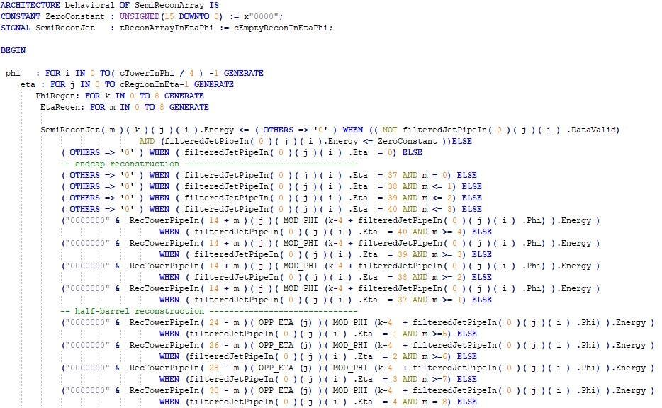
99 [86]

100 [87]

101 [88]

102 [89]

103 [90]

104 [91]

105 [92]

106 [93]

107 [94]

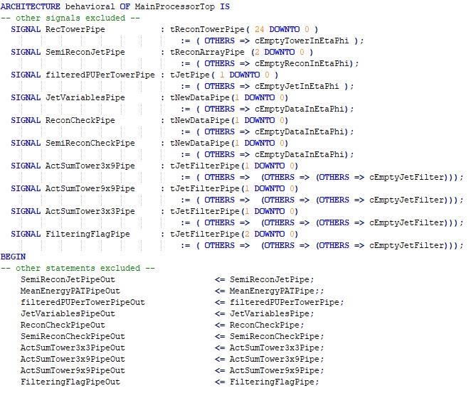
108 [95]

109 [96]

110 Appendix C2: Code Implementations/Updates for Design II [97]

111 [98]

112 [99]

113 [100]

114 [101]

115 [102]

116 [103]

117 [104]

118 [105]

119 Overall Latency of the Design I (Complete Reconstruction of Jets based on their Tower Content). Notice that for each eta the latency shown is 5 clock pulses of 250 MHz and the Semi-Reconstructed objects appear at the same time with the Reconstructed (Pile Up Subtracted) Items. The Semi-Reconstruction (Acquisition of Tower Content) begins a clock pulse prior to the one indicated, and the process used is purely for debugging purposes Appendix D: Overall Latency for the Design I (Complete Reconstruction) [106]