Βασίλειος Μαχαιράς Πολιτικός Μηχανικός Ph.D.

Transcript

1 Βασίλειος Μαχαιράς Πολιτικός Μηχανικός Ph.D. Ακέραιος προγραμματισμός πολύ-κριτηριακές αντικειμενικές συναρτήσεις Πανεπιστήμιο Θεσσαλίας Σχολή Θετικών Επιστημών Τμήμα Πληροφορικής Διάλεξη η /2017

2 Τι παρουσιάστηκε έως σήμερα Αναλυτικές μέθοδοι επίλυσης προβλημάτων βελτιστοποίησης. Μέθοδοι γραμμικού προγραμματισμού για την επίλυση προβλημάτων με γραμμική αντικειμενική συνάρτηση και γραμμικούς περιορισμούς ισότητας ή ανισότητας. Μέθοδοι επίλυσης μονοδιάστατων προβλημάτων βελτιστοποίησης, οι οποίες είναι χρήσιμες στην εύρεση του βέλτιστου μήκους βήματος σε προβλήματα επίλυσης με επαναληπτικές μεθόδους. Μέθοδοι επίλυσης μη γραμμικών προβλημάτων με και χωρίς περιορισμούς Μοντέρνες μέθοδοι βελτιστοποίησης: γενετικοί αλγόριθμοι, simulated annealing, particle swarm optimization, ant colony optimization

3 Τι θα παρουσιαστεί Μέθοδοι επίλυσης προβλημάτων με διακριτές μεταβλητές: ακέραιος προγραμματισμός Βελτιστοποίηση συναρτήσεων με πολλά κριτήρια (Multi-objective optimization)

4 Ακέραιος προγραμματισμός Μέχρι τώρα είδαμε προβλήματα με μεταβλητές απόφασης, οι οποίες είναι συνεχείς και πραγματικοί αριθμοί (ανήκουν στο σύνολο πραγματικών αριθμών R). Πολλά πρακτικά προβλήματα μπορούν να λάβουν ακέραιες αριθμητικές τιμές (διακριτές τιμές). Στις τεχνικές που παρουσιάστηκαν θα μπορούσε το πρόβλημα να επιλυθεί συμβατικά και το αποτέλεσμα να στρογγυλοποιηθεί στον κοντινότερο ακέραιο. Όμως πολλές φορές η στρογγυλοποίηση της λύσης παραβιάζει τους περιορισμούς. Αυτό μπορεί να αποφευχθεί αν προσεγγιστεί ως πρόβλημα ακέραιου προγραμματισμού.

5 Ακέραιος προγραμματισμός Όταν όλες οι μεταβλητές λαμβάνουν μόνο ακέραιες τιμές τότε ονομάζεται all-integer programming problem. Όταν λαμβάνουν μόνο διακριτές τιμές τότε ονομάζεται discrete programming problem Όταν μερικές μόνο από τις μεταβλητές λαμβάνουν ακέραιες τιμές τότε ονομάζεται mixed-integer (discrete) programming problem. Όταν οι μεταβλητές λαμβάνουν μόνο τιμές 0 ή 1 τότε ονομάζεται zero-one programming problem

6

7 Γραφική αναπαράσταση

8 Γραφική αναπαράσταση

9

10 Gomory s cutting plane method Η μέθοδος βασίζεται στη δημιουργία επιπλέον περιορισμών, ώστε να μειωθεί το αρχικό σύνολο εφικτών λύσεων με τέτοια μεθοδολογία, η οποία θα περιέχει στο όριό της τη νέα λύση ως ακέραια. Το νέο σύνολο εφικτών λύσεων που προκύπτει από τους νέους περιορισμούς πρέπει να είναι κυρτό (convex) και το τμήμα που αφαιρείται να μην περιέχει διακριτές λύσεις του προβλήματος. Οι νέοι περιορισμοί εισάγονται με συστηματικό τρόπο.

11

12

13

14

15

16

17

18

19

20 BRANCH-AND-BOUND method

21

22

23

24

25

26

27

28

29

30

31

32

33

34

35

36

37

38

39

40

41 Branch and Bound for Binary IP

42

43

44

45

46

47

48

49

50

51

52

53

54

55

56

57

58

59 Βελτιστοποίηση συναρτήσεων με πολλά κριτήρια Multi-objective optimization

60 Introduction Is an area of multiple criteria decision making, that is concerned with mathmatical optimization problem involving more than one objective function to be optimized simultaneously. Most real-world engineering optimization problems are multi-objective in nature Objectives are often conflicting Performance vs. Silicon area Quality vs. Cost Efficiency vs. Portability The notion of optimum has to be redefined

61 Multiobjective optimization (multicriteria, multiperformance, vector optimization or Pareto optimization ) Find a vector of decision variables which satisfies constraints and optimizes a vector function whose elements represent the objective functions Objectives are usually in conflict with each other Optimize: finding solutions which would give the values of all the objective functions acceptable to the designer

62 Mathematical Formulation

63 Feasible Region

64 Pareto Optimum Formulated

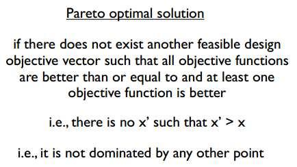
65 Pareto Optimum

66 Pareto Optimum

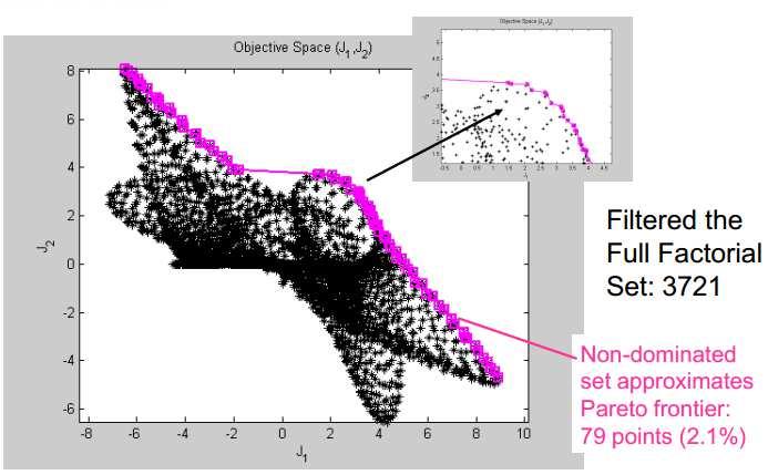
67 Pareto Front

68

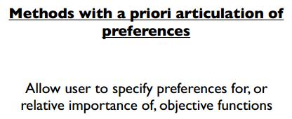
69 Multi-Objective Optimization Classic Methods : 1- Weighted Sum Method 2- Constraint method 3- Weighted Metric Methods 4- Rotated Weighted Metric Method 5- Benson s Method 5- Value Function Method Currently an Evolutionary Algorithm Methods are Used For MOOP

70 Multi-Objective Optimization All the problems that we have considered in this class have been comprised of a single objective function with perhaps multiple constraints and design variables. Minimize F(x) Subject To: g( x) 0...

71 Multi-Objective Optimization Consider the following 2D performance space: F 2 Minimize Both F s Optimum F 1

72 Multi-Objective Optimization But what happens in a case like this: F 2 Minimize Both F s Optimum? Optimum? F 1

73 Multi-Objective Optimization Suppose I wish to minimize both of the following functions simultaneously: F 1 = 750x 1 +60(25-x 1 ) x 2 +45(25-x 1 )(25-x 2 ) F 2 = (25-x 1 ) x 2 For the typical weighted sum approach, I would assign a weight to each function such that: w + w = 1 and w, w

74 Multi-Objective Optimization I would then combine the two functions into a single function as follows and solve: F T = i w F i i = w F + w F

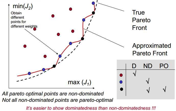
75 Multi-Objective Optimization The net effect of our weighted sum approach is to convert a multiple objective problem into a single objective problem. But this will only provide us with a single Pareto point. How will be go about finding other Pareto points? By altering the weights and solving again.

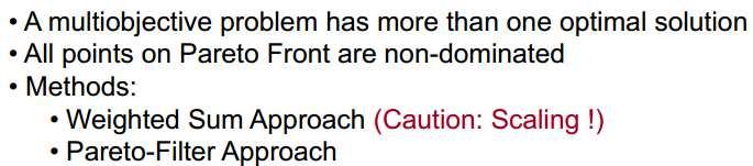
76 Multi-Objective Optimization Ok, so I march up and down my weights generating Pareto points and then I ve got a good representation of my set. Unfortunately not. As it turns out it is seldom this easy. There are a number of pitfalls associated with using weighted sums to generate Pareto points.

77 Multi-Objective Optimization Some of those pitfalls are: Inability to generate points in non-convex portions of the frontier Inability to generate a uniform sampling of the frontier A non-intuitive relationship between combinatorial parameters (weights, etc.) and performances Poor efficiency (can require an excessive number of function evaluations).

78

79

80

81

82

83

84

85