Molecular Structure: matching and kinematics

Transcript

1 Molecular Structure: matching and kinematics Ioannis Z. Emiris Dept. of Informatics & Telecoms, University of Athens Algs in Struc.BioInfo 16

2 Outline 03. Chemical bonds 06. Structure types, aminoacids, Ramachandran plot 19. Structure comparison 27. Databases, and prediction 33. Kinematics and Rigid transforms (39. Parameterization) 50. Motion planning: Configuration space 59. Degrees of freedom 64. Appendix: Energy, Ramachandran, CASP 70. Structure matching, geometric hashing 77. Protein folding 85. Docking Reading: Wikipedia for RMSD: Root-mean-square deviation. Choset, Kavraki et al. Principles of Robot Motion, Chap. 3, and E.

3 Chemical bonds

4 Chemical Bonds Covalent: Share electrons. Polar, e.g. HO, HN, HCl. Non-polar, e.g. H 2. Simple (allows rotation), or multiple (double, triple etc). Non-covalent or Ionic (or salt): transfer electrons. E.g. N acl Hydrogen: between covalently bonded H to electronegative atom, and electronegative atom, eg. O, N. Similar to non-covalent: O H O = Van der Waals: push-away A if r 3.5Å: disallows atoms to occupy same space (strong push when nearby).

5 Breakup Energy [kcal / mole] bond in void in H 2 O covalent non-covalent 90 3 H-bond Van der Waals

6 Structure types

7 Structure types Primary: ATCCGTG, FQRRTVQILQT Secondary: α-helix, β-sheet Super-secondary: α-hairpin, β-hairpin, β α β Tertiary: (3.9Å, 2.2Å, -45.1Å),.... Overall fold. E.g. N, H α, C, C β form regular tetrahedron centered at C α. Mirror symmetries isomers (proteins w/one isomer always). Quaternary: several monomers (domains) van der Waals.

8 Primary/tertiary structure of the 20 aminoacids. Backbone skeleton is: top-c, center (C α ), N-at-left. min: Glycine, special: Proline.

9 Properties of the 20 aminoacids Nonpolar not-h 2 O soluble (hydrophobic) Polar are: globally neutral, acidic(-), or basic(+). Charged are: acidic (e-acceptor) or basic (e-donor), not always polar.

10 α-helix DNA: usually B-DNA in cells, radius 10Å; Z-, A-DNA less frequent, less standard helix. Proteins: Usually right-handed spiral (αr); Sidechains usually lie inside the helix Glycine may form left-handed helix αl. Each C α advances by: 100 o, 1.5Å. i.e. 3.6 residues per turn of the helix. Rigidity by H-bonds: (C=O) i (HN) i+4, and inward hydrophobic, outward hydrophilic faces.

11 β-sheet Parallel xor antiparallel (twisted). Composed of 2 (almost) coplanar strands. φ, ψ angles differ by π. Each C α advances by: 3.5Å Rigidity due to H-bonds: C=O HN, of neighboring strands

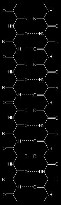
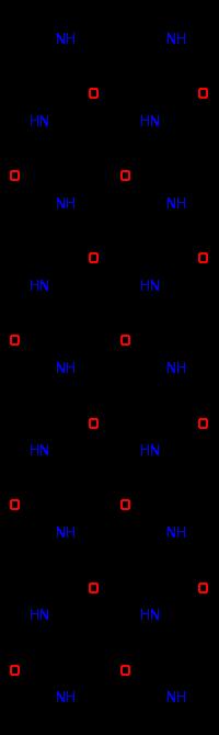
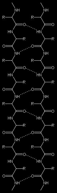
12 Antiparallel vs Parallel

13 (β-sheet variants) β-barrel: Sheet-end has right-handed twist, folds on itself. Figure: human retinol-binding protein (1RBP): 8 anti strands form barrel, binding vitamin A. If residue with 2 H-bonds bulge

14 (Rare helices) residues per turn, bind i + 4 thus narrower, longer usually at end of α-helix Π 4 residues per turn, bind i + 5 squat and constrained

15 Protein tertiary structure N, H α, C, C β form Tetrahedron, center C α. Rotation around single bonds N-C α (φ) and C α -C (ψ) one exception: proline (only ψ). angle ω around peptide bond has 2 states: trans: ω 180 o is usual cis: ω 0 o is rare, mostly at proline

16 Average rigid elements Bond Angle Mean [ o ] N-C α C o C α C-N o C-N-C α o C α N-H o Bond Length N-C α C α C C-N N-H Mean [Å] 1.46 Å 1.53 Å 1.33 Å 0.98 Å

17 Sasisekharan-Ramakrishnan-Ramachandran diagram Describes allowed mainchain conformations. Horizontal φ, vertical ψ, typically ω = 180 o. parallel β P, twisted β T ; right-handed α, left-handed L, 3 10, Π helices. Exception: Gly (no limitation), Pro (side chain back to backbone).

18 Ramachandran diagram: example structure types: α, β, Gly for protein 2ACY [Lesk].

19 Structure comparison

20 Measure difference of matched sets Hypotheses: pointsets of equal cardinality, given correspondance (match) Definition. (coordinate) Root Mean Square Deviation (c-rmsd) RMSD = 1 n n i=1 x i y i 2, where x i, y i R 3 are (C α ) atom coordinates in SAME coordinate frame. Lemma. c-rmsd satisfies the triangular inequality. Hence it defines a distance metric.

21 Optimal Alignment of matched sets Problem. Find translation and rotation minimizing c-rmsd. 1. Translate to common origin by subtracting from x i s centroid x c = 1 n n i=1 x i, x i R 3, and subtracting y c from all y i s; overall = O(n). 2. Rotate to optimal alignment by 3 3 rotation matrix Q : Q T Q = I. Also should have det Q = 1. Deterministic linear algebra (SVD) algorithm [Kabsch]: O(n). Lemma: optimal translation can be decoupled from rotation optimization. Proof: for any Q, optimal translation brings center of mass to origin.

22 Matrix algebra Let X = [x 1,..., x n ] T, Y = [y 1,..., y n ] T R n 3, then RMSD(X, Y ) = 1 n X Y F, where M 2 F = i,j M 2 ij = tr(m T M), is the Frobenius norm, tr(a) = i A ii is the trace of matrix A = [A ij ]. Recall rotated vector is v T Q or Qv, for column vector v R 3.

23 Optimal rotation Assume common centroid = 0, X, Y R n 3 : RMSD(X, Y ) = min Q Y XQ F, Q T Q = I, Q = 1. We apply: tr(a + B) =tr(a)+tr(b), tr(a) =tr(a T ), (AB) T = B T A T, Lemma A: tr(a T A) = A 2 F = AT 2 F = tr(aat ), and Lemma T: tr(ab) = ij A ij B ji = tr(ba), for A, B of equal size. Proposition. Optimizing rotation Q R 3 3 reduces to max Q tr(q T X T Y ). Proof: Y XQ 2 F = tr[(y XQ)T (Y XQ)] = = tr(y T Y ) + tr(x T X) 2tr(Q T X T Y ), where tr[(xq) T (XQ)] = tr(x T X) by Lemma A, and tr[(y ) T (XQ)] = tr[(xq) T Y ].

24 Singular Value Decomposition Recall SVD: X T Y = UΣV T, U T U = V T V = I, Σ = σ σ σ 3 where : σ 1 σ 2 σ 3, U, V, Σ are 3 3 like X T Y, and singular values σ i = e i 0, e i are eigenvalues(x T Y ). We wish to find Q that maximizes: tr(q T X T Y ) = tr(q T UΣ V T ) = tr(v T Q T UΣ) tr(σ). 2nd equality by Lem. T; inequality since M = V T Q T U is orthonormal M ij 1 tr(mσ) = i M ii σ i i σ i. Thm. Maximum occurs at M = I Q = UV T. If det Q = 1 then Q reflection, hence negate Q 33 to get rotation. Overall complexity = O(n).

25 Algorithm Input: pointsets X, Y R n 3 of n corresponding points. Output: minimum RMSD of translated and rotated sets. Algorithm. x c n i=1 x i /n, y c n i=1 y i /n. X {x x c : x X}, Y {y y c : y Y }. SVD: X T Y = UΣV T. Optional: Check σ 3 > 0, where Σ = diag[σ 1, σ 2, σ 3 ]. Q U V T. If det Q < 0 then Q [U 1, U 2, U 3 ] V T. // U i : ith column Return X Q Y F / n // or ni=1 Qx i y i 2 /n

26 distance-rmsd Assume that k distances d i, i = 1,..., k are known between point-pairs in X and between the corresponding pairs in Y, denoted d i, i = 1,..., k. Defn. For k matched distances, there is a distance-rmsd 2 = 1 k k i=1 Drawback: Computed in O(k) = O(n 2 ). (d i d i )2, k ( n 2 ). Lem. d-rmsd invariant under rigid transforms: translate, rotate, reflect. d-rmsd is a metric in (Euclidean) R r space; but then one point represents a conformation and its mirror image. Please check [Guibas?]: c-rmsd / n d-rmsd 2 c-rmsd.

27 Databases, and prediction

28 Databases Protein Data Bank (PDB) ( Structure information and retrieval File starts with protein name, author, maybe secondary structure Omits H-atoms Example: Hemoglobin, residue of Argynine: ATOM N ARG ATOM CA ARG ATOM C ARG ATOM O ARG ATOM CB ARG Protein fold classification into hierarchies: SCOP (Structural Classification of Proteins), cf next slide [Murzin et al 95, Andreeva et al 04] CATH (domains) (Class, architecture, topology, homology) [Orengo et al 97, Pearl et al 05] FSSP (DALI offers structural alignment) [Holm,Sander 96] CE (structural alignment)

29 SCOP Hierarchy Lowest level: individual protein domains (from PDB) families of homologues: similar structure, sequence, (function) imply common evolutionary origin superfamilies: families of similar structure and function, weak evolutionary relationship folds: superfamilies with common folding topology Highest level: classes: α, β, α + β, α/β (α and β) and small proteins Homology of structures expresses common ancestry: either evolutionary: evolved from structure in common ancestor (wings of bats and arms of primates), or developmental: from same tissue in embryonal development (ovaries of female and testicles of male humans).

30 SCOP example 1 Root SCOP 2 Class α/β, mainly parallel β-sheets (β α β units) 3 Fold Flavodoxin-like: 3 layers, α/β/α; parallel β-sheet of 5 strands, order Superfamily Flavoproteins 5 Family Flavodoxin-related binds FMN 6 Protein Flavodoxin 7 Species Clostridium beijerinckii [Lesk,p.224]

31 SCOP size In July 2001, SCOP contained 13,220 PDB entries, in 31,474 domains: Class families superfamilies folds All-α proteins All-β proteins α/β proteins α + β proteins Multi-domain membrane, cell-surface Small proteins Total

32 Rigid-body kinematics: Motivation

33 Molecular kinematics Given a rigid body with specific degrees of freedom (e.g. dihedral angles about covalent bonds), its kinematics describe the allowed motions under certain geometric constraints (distances, angles etc) Modeling of constraints as an algebraic / optimization problem. Applications: structure determination of small (sub)molecules, dimension-reduction during docking, pharmacophore matching. There s many small molecules: most (about 15%) with 4 dof, < 10% with > 10 dof, out of 730,000 w/rotational dof [Irwin-Shoichet 04]

34 Rigid transforms

35 Rigid (Euclidean) transformations Preserve distances and angles. Translation d R 3, x x + d. Rotation R SO(3) : R 1 = R T, det R = 1, x Rx. R 1 : rotation by negative angle. R 1 by θ 1, R 2 by θ 2 R 1 R 2 by θ 1 + θ 2. Reflection R : det R = 1 (reflection in R 2 takes body out of the plane) Scaling and Shearing are NOT rigid.

36 2D transforms Rotation, scaling, shearing: [ ] [ cos θ sin θ sx 0, sin θ cos θ 0 s y ] (typically s x, s y > 0), [ 1 a 0 1 ]. T = cos θ sin θ 0 sin θ cos θ d : homogeneous transform: translation by d, rotation (by θ) : R SO(2), R 1 SO(2), R 1 = R T, det R = 1. cos θ sin θ 0 sin θ cos θ d x y 1 i+1 = x y 1 i

37 Classification Linear transforms represented by matrix-vector multiplication: Rotation, reflection, scaling, shearing (NOT translation). They preserve linear combinations of points. Affine transform M = L + T where L is linear and T is translation. Def. 4 basic affine transforms: rotation, scaling, shearing, translation Thm. Every affine transformation written as a combination/sequence of these 4 basic affine transformations. Cor. Reflection is affine combination of 4 basics.

38 3D motion Rotation is 3 3 matrix parameterized by only 3 free elements (e.g. Euler angles in next slide, or Quaternions), not 9. Transformation between frames: cos θ sin θ cos α sin θ sin α a cos θ sin θ cos θ cos α cos θ sin α a sin θ 0 sin α cos α r Coordinate frame X i Y i Z i associated to i-th rigid link, joint allows motion between links i, i + 1. x y z 1 i+1 = x y z 1 i 4 Denavit-Hartenberg parameters (see below for details): α angle between axes Z i, Z i+1, θ about joint i (dihedral), link i of length a measured between the Z-axes, offset r at joint i 1 measured along Z i.

39 (Parameterization)

40 Rotation Matrix with Euler Angles Rotation about z0 by α + Rotation about y1 by β + Rotation about x2 by γ T 0 3 = T 0 1 T 1 2 T 2 3 = cos(α) sin(α) 0 cos(β) 0 sin(β) = sin(α) cos(α) cos(γ) sin(γ) = sin(β) 0 cos(β) 0 sin(γ) cos(γ) cos(α) cos(β) cos(α) sin(β) sin(γ) sin(α) cos(γ) cos(α) sin(β) cos(γ) + sin(α) sin(γ) sin(α) cos(β) sin(α) sin(β) sin(γ) + cos(α) cos(γ) sin(α) sin(β) cos(γ) cos(α) sin(γ) sin(β) cos(β) sin(γ) cos(β) cos(γ) [Choset,Kavraki et al. Principles of Robot Motion, Chap.E]

41 Denavit-Hartenberg Method (1955)

42 Denavit-Hartenberg Matrix For transforming two coordinate frames: Rot(Z i, θ i ) + Trans(Z i, r i ) + Trans(X i+1, a i ) + Rot(X i+1, α i ) A i = A i = cos(θ i ) sin(θ i ) 0 0 sin(θ i ) cos(θ i ) r i a i 0 cos(α i ) sin(α i ) 0 0 sin(α i ) cos(α i ) cos(θ i ) sin(θ i ) cos(α i ) sin(θ i ) sin(α i ) a i cos(θ i ) sin(θ i ) cos(θ i ) cos(α i ) cos(θ i ) sin(α i ) a i sin(θ i ) 0 sin(α i ) cos(α i ) r i X i -axis is normal to Z i and Z i 1 axes, at distance = a i 1.

43 Kinematic Chains Two types of rigid mechanisms / robots / linkages / manipulators: Serial linkage of rigid bodies connected by movable joints. Open chain, i.e. no loops. Wish to analyze motion of last link (end effector) in terms of other links. Apply Matrix multiplication: T all = T 1 T 2 T n. Parallel robots: all linkages connected to same end-effector. T 1 = = T n, where T i depends on parameters. Kinematics Problems: T i contains unknown (e.g. angle θ i ). Inverse kinematics: Given T all, compute the θ i. Trivial for parallel robots, hard for serial robots. Forward/direct kinematics: Given the T i, compute T all. Trivial for serial manipulators, hard for parallel manipulators.

44 Planar 2-R Manipulator

45 Planar 2R: parameters D-H Parameters: (stars denote variables) Link a i α i r i θ i 1 a θ 1 2 a θ 2 A 1 = Homogeneous Transformation c 1 s 1 0 a 1 c 1 s 1 c 1 0 a 1 s , A 2 = c 2 s 2 0 a 2 c 2 s 2 c 2 0 a 2 s T 0 2 = A 1A 2 = T 0 1 = A 1 c 12 s 12 0 a 1 c 1 + a 2 c 12 s 12 c 12 0 a 1 s 1 + a 2 s c 12, s 12 refer to θ 1 + θ 2.,

46 Planar 2R: kinematics Direct Kinematics x 0 = a 1 cos(θ 1 ) + a 2 cos(θ 1 + θ 2 ) y 0 = a 1 sin(θ 1 ) + a 2 sin(θ 1 + θ 2 ) θ 1 = cos 1 Inverse Kinematics y x 2 + y 2 cos 1 x2 + y 2 + a 2 1 a2 2 2a 1 x 2 + y 2 θ 2 = cos 1 x2 + y 2 a 2 1 a2 2 2a 1 a 2

47 3-Link RPP Manipulator

48 RPP: parameters D-H Parameters: (stars denote variables) Link a i α i r i θ i d 1 θ o d d 3 0 A 1 = Homogeneous Transformation c 1 s s 1 c d 1, A 2 = d 2, A 3 = d T 0 3 = A 1A 2 A 3 = c 1 0 s 1 s 1 d 3 s 1 0 c 1 c 1 d d 1 + d

49 RPP: kinematics Direct Kinematics: x 0 = sin(θ 1 )d 3 y 0 = cos(θ 1 )d 3 z 0 = d 1 + d 2 Inverse Kinematics: θ 1 = tan 1 ( x y ) d 2 = z d 1 d 3 = x 2 + y 2

50 Motion planning

51 Εισαγωγή Ερωτήματα σχετικά με τον σχεδιασμό κίνησης (motion planning) ενός ρομποτικού μηχανισμού: Πόση πληροφορία χρειάζεται για να προσδιοριστεί η θέση κάθε σημείου του ρομπότ; Πώς θα αναπαρασταθεί η παραπάνω πληροφορία; Ποιες είναι οι μαθηματικές ιδιότητες της αναπαράστασης της πληροφορίας; Πώς θα λάβουμε υπ όψιν τα εμπόδια στον σχεδιασμό των κινήσεων; [Choset, Kavraki et al. Principles of Robot Motion, Chapter 3]

52 Βασικές έννοιες Διαμόρφωση (robot configuration, molecule conformation): πλήρης προσδιορισμός της θέσης (π.χ. 3 συντεταγμένες) κάθε σημείου του ρομπότ. Χώρος διαμορφώσεων (Configuration space, C-space): Ο χώρος όλων των πιθανών διαμορφώσεων του ρομπότ, όπου καθε διαμόρφωση αντιστοιχεί σε ένα σημείο του χώρου. Βαθμοί ελευθερίας (Degrees of freedom): Ο αριθμός των παραμέτρων που απαιτούνται για να προσδιοριστεί μία διαμόρφωση. Ισοδύναμα, η διάσταση του χώρου διαμορφώσεων. Χώρος εργασίας (Workspace): Ο φυσικός χώρος που είναι προσβάσιμος από το ρομπότ, τυπικά 3Δ. Προσοχή: Χώρος εργασίας Χώρος διαμορφώσεων.

53 Παράδειγμα 1: Ρομπότ-δίσκος Ρομπότ-δίσκος, δεδομένης ακτίνας r, το οποίο κινείται στο δισδιάστατο επίπεδο R 2. Διαμόρφωση: q = (x, y) αρκεί να προσδιοριστεί το κέντρο του ρομπότ, άρα C-space R 2. Για κάθε διαμόρφωση μπορούμε να υπολογίσουμε τα σημεία που καταλαμβάνει το ρομπότ ως εξής: R(x, y) = {(x, y ) R 2 (x x ) 2 + (y y ) 2 r 2 }, r = ακτίνα του ρομπότ. Μπορούμε να ορίσουμε τον χώρο διαμορφώσεων και τον χώρο εργασίας. Είναι και οι δύο υποσύνολα του R 2, αλλά είναι διαφορετικοί!

54 Παράδειγμα 2: Βραχίονας με δύο αρθρώσεις

55 Παράδειγμα 2: Βραχίονας με δύο αρθρώσεις Διαμόρφωση: η θέση του χεριού (elbow up / down δηλ. θ 2 ) δεν αρκεί: χρειάζονται οι γωνίες και των 2 αρθρώσεων: q = (θ 1, θ 2 ). Κάθε άρθρωση μπορεί να περιστραφεί σε ένα μοναδιαίο κύκλο S 1 χώρος διαμορφώσεων Q = S 1 S 1 = T 2 δηλ. δισδιάστατος τόρος. χώρος εργασίας = ένας δίσκος R 2 (εικόνα δεξιά).

56 Εμπόδια Εμποδια χώρου διαμορφώσεων (C-space obstacles): Διαμορφώσεις q όπου το ρομπότ R(q) συγκρούεται με εμπόδιο W i : O i = {q Q R(q) W i }. Ελευθερος χώρος διαμορφώσεων (free C-space): Q free = Q \ ( i O i ) Ελεύθερο μονοπάτι (free path): Μονοπάτι χωρίς συγκρούσεις με εμπόδια που δεν περιλαμβάνει ούτε τα ακραία σημεία του Q free. Δίνεται από παραμετροποίηση: c : [0, 1] Q free. Ημι-ελεύθερο μονοπάτι (semifree path): Οπως το ελεύθερο, αλλά μπορεί να περιλαβει ακραία σημεία (όριο) του Q free : c : [0, 1] Closure(Q free ).

57 Παράδειγμα 1 (με εμπόδια) (1) Κυκλικό ρομπότ και πολυγωνικό εμπόδιο στο R 2. (2) το ρομπότ διατρέχει το εμπόδιο του χώρου εργασίας (workspace obstacle). Ελέγχουμε συγκεκριμένα σημεία. (3) Η τροχιά του κέντρου ορίζει το εμπόδιο στον χώρο διαμορφώσεων (C-space obstacle), όπου το ρομπότ = σημείο. Επαυξημένο πολύγωνο = άθροισμα Minkowski του αρχικού + δίσκο

58 Παράδειγμα 2 (με εμπόδια) A A Για τα εμπόδια στον χώρο διαμορφώσεων, θεωρούμε σύνολο διαμορφώσεων και για καθεμία υπολογίζουμε αν προκαλεί σύγκρουση. Ο βραχίονας έχει 2 αρθρώσεις: θ 1 = 0 στον άξονα x, θ 2 = 0 στον x, αμφότερες CCW. One point is fixed (center of left fig.). [Choset,Kavraki et al. Sec.3.2.2]

59 Degrees of freedom (dof) Holonomic constraints are expressed purely as a function of configuration variables (and possibly time); e.g. distances: f(q, t) = 0. For each holonomic constraint, degrees of freedom are reduced by 1: n coordinates and m holonomic constraints lead to n m dof. Non-Holonomic constraints imply not all dof are controllable, e.g. cars with 2 controls but 3 dof.

60 Planar rigid body Robot translates and rotates. A, B, C: 3 distinct points fixed to the body of robot. 6 coordinates : (x A, y A ), (x B, y B ), (x C, y C ) 3 holonomic constraints (distances): d(a, B) = (x A x B ) 2 + (y A y B ) 2 d(a, C) = (x A x C ) 2 + (y A y C ) 2 d(b, C) = (x B x C ) 2 + (y B y C ) 2 Thus, 3 dof q = (x A, y A, θ) (x A, y A ) : position of point A θ : orientation of robot Configuration space: Q = R 2 S 1

61 Open-chain jointed robot (serial mechanism) Usually, add the dof s at each joint Common joints with 1 degree of freedom revolute (R): rotating about an axis prismatic (P): translating along an axis Common joint with 3 dof s spherical (ball-and-socket)

62 Closed-chain jointed robot (parallel mechanism) 1 stationary (base) + (k 1) movable = k links System starts with N(k 1) dof (before accounting for joints): Each movable link has N dof s N = 6 for spatial mechanism N = 3 for planar mechanism Each joint places N f i constraints f i : dof s at joint i f i = 1 for prismatic/revolute joint Grübler s (or Kuzbach) formula for mobility (dof), assuming all constraints are independent: M = N(k 1) n i=1 (N f i ) = N(k n 1) + n i=1 f i.

63 Planar mechanism with 6 links: Examples B E F C A D N = 3 dof; k = 6 links A,..., F ; n = 7 revolute joints, each f i = 1. Mobility by Grübler/Kuzbach: M = 3(6 7 1) + 7 = 1 Stewart platform: 6 legs, each 5 links, 6 R/P joints. Hence k = links, n = 36 joints. Mobility by Grübler/Kuzbach M = (6 1) = 6.

64 Appendix: Chemistry, Energy, Structure

65 Chemistry basics b X a a =atomic number= #protons = # electrons, b = atomic weight= atom weight H-atom weight #protons +#neutrons. weight of H-atom = 1 dalton := g. 1 mole = Avogadro atoms = atoms = b g. Atoms with common a and different b are isotopes: 1 H 1, 12 C 6, 14 N 7, 16 O 8, 31 P 15, 32 S 16, 39 K 19.

66 Total Energy Total potential (for Molecular Mechanics) is the sum of the following: Covalent bonds: length of bond b, where standard len 0 : c b (len b len 0 ) 2, angle between bonds, standard angle θ 0 : c a (θ a θ 0 ) 2, dihedral angle φ i, standard φ 0 : c i (1 + cos(φ i φ 0 )). Non-bond interaction (i, j) ( Lennard-Jones (mainly van der Waals): D ij ( c ij r ) 12 ( c ij ij electrostatic: r ij = distance, q i = charge: q i q j e r e 0 r ij. r ij ) 6 ), Constants: c b 500 kcal/mole, c a 5 kcal/mole, Dielectric Constant = e r e 0.

67 Ramachandran diagram (stats) 20-residue average except Gly / Pro

68 (Tertiary) structure determination Modeling geometry flexibility (required by function) n backbone residues (say 100), k 3 conformations each = molecules However nature finds favorable conformation, fast (Levinthal s paradox)

69 CASP benchmark Critical Assessment of Structure Prediction Organizes blind test of protein structure, given sequence. Runs on a two year cycle. Experimental results are kept secret until predictions are submitted. secondary structure: helix H, (extended) strand E, other 3D structure predicted by assembling predicted helices, strands of sheet [Janin]

70 Structure matching

71 Rigid Matching Finding best transform ie. yielding max/bio-favorable superposition. Dependent on sequence-order: Matching set [Taylor-Orengo 89] (Dynamic Programming SSAP). fragments [Vriend-Sander] follow sequence order. FSSP-DALI [Holm,Sander 93], CE [Bourne,Shindyalov 98] Independent of Sequence (unlabeled points, different cardinalities) Geometric hashing (from vision): finds translation, rotation, scaling maxclique in SSE graph (by 2ary elements) [Mitchel et al] [Koch et al] Sequence independence: - 3d task vs essentially linear task. - Simultaneous match of sequence / structure is better + Finds non-sequential motifs eg. binding sites + works with partial / disconnected input

72 Geometric Hashing: 2D preprocess Preprocess each pointset (model) in database: pair (points #4, #1 below), define a reference frame: Compute coordinates (x, y) of all points in this frame, store [model, frame] in entry Hash(x, y). Storing 3 hash entries (2 shown by arrows) in 2D

73 Geometric Hashing: 2D query Online processing of query pointset (image): I. Pick reference frame (defined by 2 points): compute coordinates of all query points in this frame. II. Hash query points: for every data point in its hash-entry, cast a vote for the corresponding [model, frame] III [model, transform] with high scores induce potential match: optimize transform by least-squares (or RMSD on matched points) Hashed points vote for each [model,frame] pair in their hash entries (2 arrows shown)

74 Geometric Hashing: Complexity Parameters. M = #structures in database (models), n = #points per structure/model, c = 1 + #points to define a frame: c = 3 in 2D, c = 4 in 3D. Time complexity. preprocess = O(Mn c ), online query = O(Hn c ), where H = #complexity of checking one hashtable entry. H = O(1) typically when Space = O(Mn c ), good hashing; or can be H = O(Mn c ) for small/unlucky tables. [eclass/eggrafa/apallaktikh/wolfson-rigoutsos 99]

75 Geometric hashing: generalization Idea: Given two objects each with n unlabeled points: Each Pair of almost-congruent triangles defines 3D rigid transform (congruent/similar: invariant under translation, rotation, scaling) For each candidate transform, count superposed points. For best candidates, find RMSD on matched pairs, keep the best. Complexity O(n 7 ) (if we exploit backbone geometry: n 3 ) [Wolfson slides] Against database: 0. point (residue), define local neighborhood. 1. Geometric Hashing gives seed matches. 2. Cluster seed matches by merging matched points 3. Compare RMSDs of clusters; extend better clusters until solution Extra: store features into [model, frame, features]

76 Flexible Alignment Motivation. Mutations/docking imply conformational change Hinge and shear motion of domains [Lesk] Existing work 3D curve matching [Schwartz,Sharir 87], using splines [Wolfson et al 91] Dock [Leach,Kutz]. FlexX (dock), FlexS (structures) use anchors [Lengauer,Lemmen,Klebe 98] small-molecule database search [Rigoutsos,Platt,Califano 96] Pose clustering [Verbitsky,Wolfson,Nussinov 99]. Known hinges, hashing [Fligelman,Nussinov,Wolfson 00] FlexProt [Shatsky,Nussinov,Wolfson 02]

77 Optional further topics

78 Protein folding

79 Folding Protein folding: process by which a polypeptide folds from its mrna unfolded state into its native state, i.e. characteristic (and functional) 3D structure. Result determined by amino acid sequence. This is Anfinsen s, or 2nd, dogma [Anfinsen 73]

80 Folding factors Folding depends on solvent (water or lipid bilayer) concentration of salts temperature presence of molecular chaperones [Lee,Tsai 05] Folding is affected by external fields (electric, magnetic) molecular crowding, limitation of space.

81 Disruption of the native state Proteins denaturate: thermally unstable: high/low temperatures solutes, extremes of ph, mechanical forces, chemical denaturants Denatured protein: random coil, no secondary or tertiary structure. Chaperones: protect from denaturation; help to fold. Incorrect folding and aggregated proteins cause: prion-related illnesses amyloid-related illnesses familial amyloid cardiomyopathy or polyneuropathy intracytoplasmic aggregation diseases proteopathy diseases Therapy: protein replacement, pharmaceutical chaperones

82 Folding speed Levinthal s paradox [Levinthal 68]: Folding is NP-hard. fast! (through a series of intermediate states) Yet, proteins fold proline isomerization: minutes or hours small single-domain proteins: milliseconds or microseconds

83 Computational methods Energy landscape: principle of minimal frustration describes protein folding by leveling the free-energy landscape high-dimensional phase-space where manifolds take several topological forms [Robson,Vaithilingham 08] supported by computational simulation of model proteins, and experimental studies [Bryngelson,Onuchic,Socci,Wolynes 95]

84 Modeling of protein folding Molecular Dynamics (MD): studying protein folding and dynamics in silico. First: implicit solvent model and Umbrella Sampling. High computational cost: with explicit water peptides and very small proteins. larger proteins only dynamics of the structure or high-temperature unfolding long-time folding processes approximations or simplifications in protein models (pseudo-atoms representing groups of atoms) Distributed computing projects: project.

85 Docking

86 Definitions Receptor: receiving molecule, usually protein or other biopolymer. Ligand: complementary partner molecule, binds to receptor; most often small molecules but could be another biopolymer. Docking: simulation of candidate ligand binding to receptor. Binding mode: orientation of ligand relative to receptor and conformation of ligand and receptor when bound together. Pose: a candidate binding mode. Scoring: process of evaluating particular pose by counting number of favorable intermolecular interactions e.g. hydrogen bonds, hydrophobic contacts. Ranking: classifying which ligands are most likely to interact favorably to particular receptor based on predicted free-energy of binding.

87 Significance of Docking Predicting: strength of association (binding affinity) between two molecules; strength and type (e.g., agonism vs antagonism) of signal; binding orientation of small molecule drug candidates to their protein targets. Docking: computationally simulate the molecular recognition process. optimized conformation and relative orientation for protein and ligand s.t. the free energy is minimized.

88 Docking approaches Shape complementarity: matching technique that describes the protein and the ligand as complementary surfaces. [Goldman,Wipke 00], [Meng,Shoichet,Kuntz 04], [Morris,Goodsell,Halliday,Huey,Hart,Belew,Olson 98] Simulation: simulate the actual docking process in which the ligand-protein pairwise interaction energies are calculated [Feig,Onufriev,Lee,Im,Case,Brooks 04]

89 Shape complementarity Describe that makes protein and ligand dockable [Shoichet,Kuntz,Bodian 04]: Molecular surface/ complementary surface: receptor - solvent-accessible surface area, ligand - matching surface Hydrophobic features of the protein: turns in the main-chain atoms. Fourier shape descriptor technique [Cai,Shao,Maigret 02], [Morris,Najmanovich,Kahraman,Thornton 05], [Kahraman,Morris,Laskowski,Thornton 07] Advantages: fast and robust; scalable to protein-protein interactions; amenable to pharmacophore based approaches. Disadvantage: cannot accurately model the movements or dynamic changes.

90 Simulation Protein and ligand are separated by some physical distance, ligand finds its position into the protein s active site after a certain number of moves. After each total energy of the system is calculated. Moves: translations rotations internal changes to the ligand s structure (incl. torsion angle rotations) Advantages: easy to incorporate ligand flexibility; process physically closer to reality. Disadvantage: slow

91 Mechanics of docking Determine structure of the protein by X-ray crystallography NMR spectroscopy Docking program: search algorithm scoring function

92 Search algorithm Search space: all possible orientations and conformations of protein paired with ligand. enumerate all possible distortions of each molecule, all possible rotational and translational orientations of the ligand relative to the protein. In practice: flexible ligand (most programs) flexible protein receptor Search Strategies: systematic or stochastic torsional searches about rotatable bonds molecular dynamics simulations genetic algorithms to evolve new low energy conformations

93 Ligand flexibility Conformations of the ligand may be generated without receptor, then docked [Kearsley,Underwood,Sheridan,Miller 94] on-the-fly in the presence of the receptor binding cavity [Friesner et al 04] with full rotational flexibility of every dihedral angle (fragment based docking) [Zsoldos,Reid,Simon,Sadjad,Johnson 07] Select low energy conformations: force field energy evaluation (usual) [Wang,Pang 07] knowledge-based methods [Klebe,Mietzner 94]

94 Receptor flexibility large number of degrees of freedom [Cerqueira,Bras,Fernandes,Ramos 09] Emulate receptor flexibility: Multiple static structures for the same protein in different conformations [Totrov,Abagyan 08] Rotamer libraries of amino acid side chains that surround the binding cavity [Hartmann,Antes,Lengauer 09], [Taylor,Jewsbury,Essex 03]

95 Scoring function Input: pose ( snapshot of ligand + protein) Output: number (likelihood of binding) Scoring functions analyze: energy of the pose (physics-based molecular mechanics force fields): a low (negative) energy likely binding interaction potential fit of the pose (databases of protein-ligand complexes)

96 Using Databases X-ray crystallography: Many: proteins + high affinity ligands Less: proteins + low affinity ligands false positive hits Solution: recalculate the energy of the top scoring poses (Generalized Born, Poisson-Boltzmann [Feig,Onufriev,Lee,Im,Case,Brooks 04])

97 Applications Hit identification: docking combined with scoring function used to quickly screen large databases of potential drugs to identify molecules that are likely to bind to protein target of interest (virtual screening). Lead optimization: predict where and in which relative orientation a ligand binds to a protein (binding mode or pose). Bio-remediation: predict pollutants that can be degraded by enzymes [Suresh,Kumar,Kumar,Singh 08].