NON-LINEAR OPTICS AND QUANTUM OPTICS

Transcript

1 NON-LINEAR OPTICS AND QUANTUM OPTICS Non classical states squeezed states (degenerate parametric down conversion and second harmonics generation) entangled states (non-degenerate parametric down conversion ) conditional states Non-linear beam splitter (sum frequency generation)

2 Classical BIBLIOGRAPHY Y.R. Shen The principles of nonlinear optics John Wiley & Sons (New Yor, 984) M. Schubert, B. Wilhelmi Nonlinear optics and quantum electronics John Wiley & Sons (New Yor, 986) V.G. Dmitriev, G.G. Gurzadyan, D.N. Niogosyan Handboo of nonlinear optical crystal Springer- Verlag (Berlin Heidelberg, 990) P.N. Butcher, D. Cotter The elements of nonlinear optics Cambridge University Press (Cambridge, 990) B.E.A. Saleh, M.C. Klein Fundamentals of photonics John Wiley & Sons (New Yor, 99) A.C. Newell, J.V. Moloney Nonlinear optics Addison-Wesley (Redwood City, 99) D.L. Mills Nonlinear optics Springer-Verlag (Berlin Heidelberg, 99) Handboo of Photonics Editor-in-Chief M.C. Gupta - CRC Press (Boca Raton New Yor, 997) R.W. Boyd Nonlinear optics Academic Press (San Diego, 99) G.S. He, S.H. Liu Physics of nonlinear optics World Scientific (Singapore, 999) Quantum L. Mandel and E. Wolf Optical coherence and quantum optics Cambridge University Press (Cambridge, 995) R. Loudon The quantum theory of light (third edition) Oxford University Press (Oxford, 000) U. Leonhardt Measuring the quantum state of light Cambridge University Press (Cambridge, 997)

3 MAXWELL EQUATIONS IN DIELECTRIC MEDIA E P E = µ 0 c0 t t D B H= ; E= t t D= 0 ; B= 0 D= ε E+ P ; B= µ H 0 0 for homogeneous and isotropic media we can derive a wave equation if the medium is wealy nonlinear, we can write: P= εχe+ de + 4 χ E +... = εχe+ P and thus: () 0 0 NL where c 0 is the propagation velocity in vacuum E P = c t t NL E µ 0 where c is the propagation velocity in the medium Second-order nonlinear optics P NL = de Third-order nonlinear optics P NL = 4χ E ()

4 Second-order nonlinear optics COUPLED-WAVE THEORY OF THREE-WAVE MIXING E PNL E = µ 0 with P NL() t = de () t c t t Er iω qt iωqt iωqt (, t) = E ( ) e + E ( ) e = E ( ) e with ω = ω ; E = E r r r * * q q q q q q q q=,, q=±, ±, ± = i( q r) t PNL ( r, t) d Eq( r) Er( r ) e ω + ω NL = d ( ω + ω ) qr, =±, ±, ± If we suppose that the three waves interacting in the medium, have distinct frequencies ω, ω and ω, and one frequency is the sum or the difference of the other two, (frequency matching condition ω = ω + ω ) we get three equations: ω + = c ω + = c ω + = µ ω + ω c * µ 0 ( ω ω ) iωt Ee d EEe * µ 0 ( ω ω ) iωt Ee d EEe ( ) iωt Ee d EEe 0 ( ω ω ) i ( ω ω ) i ( ω + ω ) i t t t P t qr, =±, ±, ± q r q r i( ωq+ ωr) E E e Nondegenerate three-wave mixing ( * ) E( r) = µ 0dωE( r) E( r) ( * ) E( r) = µ 0dωE( r) E ( r) ( ) E( r) µ 0dωE( r) E( r) = Degenerate three-wave mixing ω = ω ( * ) E( r) = µ 0dωE( r) E ( r) ( ) E( r) µ 0dωE( r) E( r) + + = t

5 COLLINEAR THREE-WAVE MIXING: PLANE-WAVE SOLUTION ( r) = ( ) = η ω ( ) E E z a z e i z q q q q q q iz ( q ωqt) * iz ( q ωqt) t = q q aq z e aq( z) e + (, ) η ω ( ) Er q=,, η 0 η q = = nq ε µ 0 0 n q Eq ( z) ( ) = = ω ( ) φ ( z) Iq z q aq z η q q I ( z) q = = ω q a q ( ) z photon flux density [ph/(s m )] We suppose that the envelope a q (z) is slowly varying with z and use the slowly varying envelope approximation (SVEA) ( ) q q( ) i z q + = da dz da dz da dz a z e = iga a e * = iga a e * = iga a e i z i z i z dz SVEA daq i where da a q q q q dz g d iqz daq + a q q e iq e dz ωωω = η 0 nnn = i z q coupling coefficient detuning

6 PARAMETRIC APPROXIMATION undepleted reference field a (z) = a (0) : da dz da dz = * i z z a( 0) a( 0 ) z a( z) = e a( 0cos ) + + i sin + + i z z a( 0) a( 0 ) + z a( z) = e a( 0cos ) + i sin + + undepleted pump a (z) = a (0) : da dz da dz = iga = = iga a iga * iga a ( 0) * ( 0) ( 0) ( 0) a e a e * e e i z i z i z i z ga ga ( ) 0 = ( ) 0 = * da = i ae dz da = i ae dz da * = i ae dz da * = i ae dz i z i z i z * i z z a( 0) a( 0 ) z a( z) = e a( 0cosh ) + i sinh * i z z a( 0) a( 0 ) z a( z) = e a( 0cosh ) i sinh + i z

7 UNDEPLETED REFERENCE FIELD up-conversion: a (0) 0 ; a (z) = a (0) ; a (0) = 0 z z a z = a + + i + e a( 0) i z z a( z) = i sin e + + i ( ) ( 0) cos sin + z Photon-flux densities Phases z φ( z) = φ( 0) cos z φ( z) = φ( 0) sin + + z Λ ( z) = Λ ( 0) + arctan tan + z + π Λ ( z) = Λ ( 0) +Λ( 0 ) + z

8 fl up-conversion in phase matching : z φ( z) = φ( 0cos ) z φ( z) = φ( 0sin ) The efficiency of up-conversion is: ( z) ( 0) Λ = Λ π Λ ( z) =Λ ( 0) +Λ ( 0) I ( z) ( ) K = = I z sin 0

9 fl up-conversion with phase mismatch : K sin I ( z) z + I ( 0) 4 z + = = z the effect of the the phase mismatch is the reduction of the conversion efficiency: For wea coupling z sinc z K z sin I ( z) z I ( 0) 4 z = = π π π π z

10 UNDEPLETED REFERENCE FIELD down-conversion: a (0) = 0 ; a (z) = a (0) ; a (0) 0 ( 0) * a z i z a( z) = i sin e + + z z a z a i e i ( ) = ( 0) cos + sin + + z Photon-flux densities Phases z φ( z) = φ( 0) sin + + z φ( z) = φ( 0) cos π Λ ( z) = Λ ( 0) Λ ( 0 ) z z Λ ( z) = Λ( 0) arctan tan + + z +

11 UNDEPLETED PUMP a (0) 0 (signal) ; a (0) = 0 (idler) ; a (z) = a (0) (pump) z z a z = a + i e * a( 0) i z z a( z) = i sinh e i ( ) ( 0) cosh sinh z Photon-flux densities Phases z φ( z) = φ( 0) + sinh z φ( z) = φ( 0) sinh z Λ ( z) = Λ ( 0) + arctan tanh z π Λ ( z) = Λ( 0) Λ( 0 ) z

12 UNDEPLETED PUMP fl parametric amplification in phase matching >, = 0: z φ( z) = φ( 0cosh ) Λ ( z) = Λ( 0) π z φ( z) = φ( 0sinh ) Λ ( z) =Λ ( 0) Λ ( 0) I ( z) z The efficiency of parametric amplification is: K = = cosh I 0 ( ) fl parametric amplification out of phase matching á, 0 : z ( ) ( 0 ) z e φ z φ + e 4 The signal amplification is: ( ) ( 0) I ( ) z I z I z z e Γ= = e =Γ = 0e 0 4

13 UNDEPLETED PUMP < z tan z φ( z) = φ( 0) sin ; ( z) ( 0) arctan + z Λ = Λ + z π φ( z) = φ( 0) sin ; Λ ( z) =Λ( 0) Λ( 0 ) z fl parametric generation of superfluorescence Ü : φ z ( z) φ( 0) + sin The signal amplification is: z z sin sin I( z) I( 0) z z Γ= sin 0 I ( 0) = = =Γ 4 z z

14 PHASE MATCHING The efficiency of the parametric processes is maximum in condition of phase matching fl nonlinear materials in which the phase mismatch can be modified. FREQUENCY MATCHING ω = ω + ω PHASE MATCHING = + collinear ( ) = ( ) + ( ) ω n ω ω n ω ω n ω θ θ θ θ non collinear ω n( ω) cos θ = ω n( ω) cos θ+ ω n( ω) cosθ ω n( ω) sin θ = ω n( ω) sin θ+ ω n( ω) sinθ OPTICALLY ANISOTROPIC CRYSTALS as the nonlinear media UNIAXIAL and BIAXIAL crystals

15 UNIAXIAL CRYSTALS Characterized by the presence of a special direction called optical-axis (Z-axis). The plane containing the Z-axis and the wave vector is called the principal plane. X Z α The refractive indices of the ordinary (n o ) and extraordinary (n e ) beams in the plane normal to the Z-axis are called the principal values. Y n e > n o positive crystal n o > n e negative crystal The light beam whose polarization is normal to the principal plane is called ordinary beam (o-beam) The light beam whose polarization is parallel to the principal plane is called extraordinary beam (e-beam) E 90 E Z E 90 E Z The refractive index n o of the o-beam does not depend on the propagation direction Note that in general n o = n o (ω) ; n e = n e (ω) and they are given by dispersion relations such as Sellmeier relations The refractive index n extr of the e-beam depends on the propagation direction being a function of the angle θ between the Z axis and the vector : n cos θ sin θ extr = + no ne

16 PM I : ω Æo, ω Æ o, ω Æ e ω = ω+ ω ω n( ω, α) cos θ = ω n( ω) cos θ+ ω n( ω) cosθ ω n( ω, α) sin θ = ω n( ω) sin θ+ ω n( ω) sinθ n( ω) = no( ω) n( ω) = no( ω) cos α sin α n( ω, α) = + no ( ω) ne ( ω) PM II PHASE-MATCHING CONDITIONS uniaxial crystals d = d α ϕ eff cos cos Optimization for PM II: crystal cut at ϕ = 0 PM I d = d sinα d cosα sin ϕ eff 5 Optimization for PM I: crystal cut at ϕ = 90 PM II : ω Æo, ω Æ e, ω Æ e ω = ω+ ω ω n( ω, α) cos θ = ω n( ω) cos θ+ ω n( ω, θ, α) cosθ ω n( ω, α) sin θ = ω n( ω) sin θ+ ω n( ω, θ, α) sinθ n( ω) = no( ω) cos ( α θ) sin ( α θ) n( ω, θ, α) = + no ( ω) ne ( ω) cos α sin α n( ω, α) = + no ( ω) ne ( ω)

17 Many possible phase-matched interactions depending on the angles between the fields, on the wavelength and on the tuning angle θ θ θ θ

18 5 (deg) ( θ θ ) ( θ θ ) Internal phase-matching angles in BBO I for λ = 0.49 µm (deg) α = α (deg) λ ( µ m) External phase-matching angles (deg) α = 4, θ cut = 4 (deg) α = 4, θ cut = λ ( µ m) -0 λ ( µ m)

19 NON COLLINEAR TYPE I INTERACTION SCHEME y x X 0 E E ϑ Fields Y optical axis ϑ xˆ η0 ω E( r, t) = { a( r) exp i( t) cc..} n r ω + xˆ η0 ω E( r, t) = a( r) exp i( ωt) cc.. n r + wˆ η0 ω E( r, t) = a( r) exp i( ωt) + cc.. n r ϑ E α { } { } Z z Parameters g = d +, +, eff Phase mismatch = d = d cosα + d + d = d sinα d sinα cosα ωωωη 0 g = g+ + g ( ω) ( ω) ( ω, α) n n n ( cosα sinα) g = d + d ωωωη 0 n( ω) n( ω) n( ω, α) ( r) = ( r) + ( r) g a g a g a eff + y z ( ˆ ) ( ˆ ) wˆ = yˆ g + z g g + g = yˆ g + z g g + + +

20 MAXWELL EQUATIONS For non-collinear type I interaction out of phase matching undepleted pump a (r) = a (0): ˆ a r = ig a r a r exp i r ˆ a r = igeff a r a r exp i r ˆ g a r = i a r a r exp i r geff * ( ) eff ( ) ( ) ( ) * ( ) ( ) ( ) ( ) ( ) ( ) ( ) ( ) ˆ i ˆ ˆ ˆ ˆ * ia a( r) = a( 0) coshq r + sinhq r + a ( 0) sinh Q exp i Q ˆ ˆ r Q r ˆ i ˆ ˆ ˆ ia ˆ a ( r) = a ( 0) cosh Q r + sinh Q r + a ( 0) sinh Q r exp i r * Q ˆ ˆ Q in phase matching = 0 and ˆ ˆ ˆ ˆ ˆ ˆ = ˆ = A g a ( ) = 0 eff A ( ) ( ) ˆ * iλ + π / A ( ) ˆ a r = 0cosh 0 sinh PM a r ˆ ˆ + a e r ˆ ˆ A * / ( ) ( 0cosh ) ˆ iλ + π A a a a ( 0) e sinh ˆ r = + PM r ˆ ˆ r ˆ ˆ 4 A Q= ( ˆ ˆ )( ˆ ˆ )

21 QUANTUM DESCRIPTION OF THE PROCESSES Three-wave mixing ω < ω < ω H= κ ( aaa ˆ ˆ ˆ + aaa ˆ ˆ ˆ ) = exp τ ( ˆˆˆ + ˆˆˆ) { } U i aa a a a a quantum Hamiltonian Evolution operator The Heisenberg equations of motion derived by the quantum Hamiltonian correspond to the classical Maxwell equations daˆ = a ˆ, H = iκ a ˆ a ˆ dt i daˆ ˆ, ˆ = a H = iκ a a ˆ dt i daˆ = a ˆ, H = iκ aa ˆ ˆ dt i Note that the coupling coefficient depends on all the parameters of the interaction, possibly including the phase mismatch By mapping time evolution into spatial evolution, we obtain that quantum equations are formally equivalent to classic equations, for operators instead of field-amplitudes

22 SPONTANEOUS DOWN CONVERSION If we now consider the Hamiltonian for undepleted pump field, that can be analytically solved, we get H = κ( * aa ˆˆ ˆˆ + aa ) { } ( τ ) = exp τ ( * ˆˆ + ˆˆ ) U S i i aa a a daˆ dt daˆ dt = = iκaˆ iκ aˆ * iφ iφ * ( 0cosh ) [ κ ] ( 0) sinh[ κ ] µ ( 0) ν ( 0) * iφ iφ * ( ) [ κ ] + ( ) [ κ ] = µ ( ) + ν ( ) aˆ = aˆ t + aˆ e t = aˆ + e aˆ aˆ= aˆ 0 cosh t aˆ 0 e sinh t aˆ 0 e aˆ 0 µ ν = which is the two-mode squeezing transformation originating the twin-beam twb = n= 0 n ψ ξ ξ n n ξ = i ν e φ µ where we can identify κ t A ˆ r ˆ ˆ

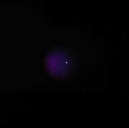
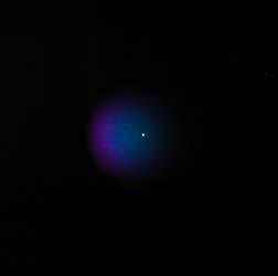
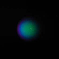
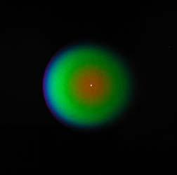
23 Experimental system to generate spontaneous down conversion: TWA = travelling-wave optical parametric amplifier Laser Nd:YLF L 49 nm BBO Laser Nd:YLF laser mode-loced, amplified λ F = 047 nm, λ SH = 5 nm, λ TH = 49 nm Pulse time duration nm, Energy per pulse 60 µj, rep-rate 500 Hz Crystal β-bab O 4 (BBO) Cut for type I (ooe) interaction θ cut =.8 Dimensions 0 0 mm

24

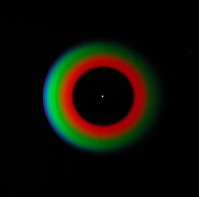
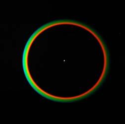
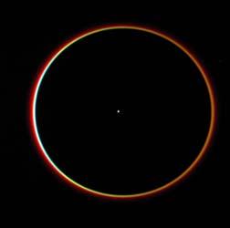
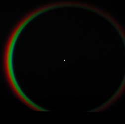
25

26 Experiment Simulation

27 STATISTICAL PROPERTIES The state of a quantum system is fully described by the statistical operator ρ ρ can be represented on different bases, such as - on the number states (Foc states) - on the coherent states -P representation where P(α) is real and normalized ρ = = π nm, = 0 n n ρ m m ρ α α ρ β β d αd β P = ρ P( α) α α d α ( α) d α = but it is not positive in all cases, so that it cannot be interpreted as a probability distribution in classical sense. Moreover P(α) sometimes does not exist.

28 The P-representation exists if and only if the Fourier transform of the normally-ordered characteristic function,, exists { a a} * * * η η ηα η α χ ( η) ρ ( α) α = N tr e e e P d if the P-representation exists * * P( ) = e ( ) d π ηα ηα α χ N η η Alternatively we can use the simmetric characteristic function { a a ρ } * χη ( ) tr e η η * * W( ) = e ( ) d π ηα ηα α χη η If the P-representation exists, we have χ ( ) N η and define the Wigner function α α' W( α) = e P( α) d α' π

29 PARAMETRIC DOWN CONVERSION Statistical properties of one of the fields produced/amplified by the TWA ) Initial state for fields and is a pure coherent state α0, α0 ρ = α0, α0 α0, α0 ( ) ( ) aˆ () t = aˆ 0 µ + aˆ 0ν * * χ N ( η) = exp η ν + ηα η α α being the mean value of α α P( α) = exp πν ν α α( t) W ( α) = exp + + ν π ( ν ) Photon number distribution ( ) p n n ( ν ) α L n n+ ( ν ) ( ) α = exp ( + ν ) + ν + ν â

30 ) Initial state for fields and is the vacuum state α0 α0 = 0, = 0 α P( α) = exp πν ν α W ( α) = exp π ( + ν ) + ν Photon number distribution ( ) p n = n ( ν ) ( + ν ) n+

31 The Wigner function can be reconstructed by optical tomography that maes use of the data from homodyne detection complete information about the quantum state all the elements of the density matrix The photon number distribution can be obtained from the Wigner function, but it can also be measured separately, without maing use of homodyne detection partial information about the quantum state only the diagonal elements of the density matrix

32 There are many different features of classical and quantum states that can be used for characterizing them: - with respect to the Wigner function: Gaussian or non gaussian-states tomographic reconstruction of the Wigner function - with respect to the photon number distribution: Poissonian, sub-poissonian and super-poissonian states direct measurement of the Fano factor F σ = n ( n)