Spectroscopic Classification of ULIRGs SWIRE sources

Transcript

1 ARISTOTLE UNIVERSITY OF THESSALONIKI SCHOOL OF NATURAL SCIENCE - PHYSICS DEPARTMENT SECTION OF ASTRONOMY, ASTROPHYSICS AND MECHANICS Spectroscopic Classification of ULIRGs SWIRE sources Diploma Thesis By Kalfountzou Eleni Supervisors Dr. Markos Trichas, Imperial College London, UK Prof. John H. Seiradakis, Aristotle University of Thessaloniki, Greece

2 Aristotle University of Thessaloniki Department of Physics Section of Astrophysics, Astronomy and Mechanics To my lovely grandmother, Stella Koutsiari.

3

4 Abstract The goal of my Diploma Thesis was the study of a sample of U/HLIRGs in the SWIRE CDFS field. The sample was observed using multi-object spectroscopy with EFOSC2 on the ESO 3.6m Telescope. Data were reduced using IRAF. I was able to estimate reliable redshifts for 54 sources out of 62. The redshift for 3 of these sources was estimated equal to 0. The spectroscopic redshifts were compared to the estimated values of photometric redshifts using the latest version of the ImpZ code (Rowan- Robinson et al 2008). Emission line diagnostics were used for 17 of sources to distinguish AGN from star-forming sources and LINERs and the results were compared to the predictions of SED template fitting methods and mid-ir diagnostics. From the 5 sources which are best fitted with a cirrus IR-template, 3 are classified as pure star-forming sources, 1 as an AGN and 1 composite. From the 7 sources which are best fitted with a starburst IR- template, 5 are classified as pure star-forming sources, 1 as LINER and 1 as ambiguous. From the 4 sources which are best fitted with a torus IR- template, 2 are classified as an AGN, 1 as a composite (torus component contributing 60%, starburst contributing 40%) and 1 as composite with LINER presence. The last two sources have no excess in the IR SED fitting but are classified as composite. iv

5 Contents Contents... v List of Figures...viii List of Tables...xiii ΜΕΡΟΣ Α... Σθάικα! Δελ έρεη νξηζηεί ζειηδνδείθηεο. Κεθάλαιο 1... Σθάικα! Δελ έρεη νξηζηεί ζειηδνδείθηεο. Ειζαγυγή... Σθάικα! Δελ έρεη νξηζηεί ζειηδνδείθηεο. 1.1Πεπίλητη... Σθάλμα! Δεν έσει οπιζηεί ζελιδοδείκηηρ. 1.2Γαλαξίερ... Σθάλμα! Δεν έσει οπιζηεί ζελιδοδείκηηρ Starburst... Σθάλμα! Δεν έσει οπιζηεί ζελιδοδείκηηρ AGN (Ενεπγόρ Γαλαξιακόρ Πςπήναρ)Σθάλμα! Δεν έσει οπιζηεί ζελιδοδείκηηρ. 1.3Αζηπονομία ζηο ςπέπςθπο... Σθάλμα! Δεν έσει οπιζηεί ζελιδοδείκηηρ. 1.4Φαζμαηοζκοπία... Σθάλμα! Δεν έσει οπιζηεί ζελιδοδείκηηρ Η Φαζμαηοζκοπία ζηην ΑζηπονομίαΣθάλμα! Δεν έσει οπιζηεί ζελιδοδείκηηρ CCD θαζμαηοζκοπία.. Σθάλμα! Δεν έσει οπιζηεί ζελιδοδείκηηρ. Κεθάλαιο 2... Σθάικα! Δελ έρεη νξηζηεί ζειηδνδείθηεο. Παπαηηπώνηαρ ζηο ςπέπςθπο. Σθάικα! Δελ έρεη νξηζηεί ζειηδνδείθηεο. 2.1Πεπίλητη... Σθάλμα! Δεν έσει οπιζηεί ζελιδοδείκηηρ. 2.2Αποζηολέρ για παπαηήπηζη ζηο ςπέπςθποσθάλμα! Δεν έσει οπιζηεί ζελιδοδείκηηρ Infrared Astronomy Satellite (IRAS)Σθάλμα! Δεν έσει οπιζηεί ζελιδοδείκηηρ ISO (Infrared Space Observatory)Σθάλμα! Δεν έσει οπιζηεί ζελιδοδείκηηρ AKARI... Σθάλμα! Δεν έσει οπιζηεί ζελιδοδείκηηρ Spitzer Space TelescopeΣθάλμα! Δεν έσει οπιζηεί ζελιδοδείκηηρ. 2.3SWIRE... Σθάλμα! Δεν έσει οπιζηεί ζελιδοδείκηηρ Επιλογή ηυν πεδίυν παπαηήπηζηρσθάλμα! Δεν έσει οπιζηεί ζελιδοδείκηηρ Ανηικείμενο μελέηηρ ηος SWIREΣθάλμα! Δεν έσει οπιζηεί ζελιδοδείκηηρ. 2.4Υπέπςθποι γαλαξίερ... Σθάλμα! Δεν έσει οπιζηεί ζελιδοδείκηηρ Ultraluminous Infrared Galaxies (ULIRGs)Σθάλμα! Δεν έσει οπιζηεί ζελιδοδείκηηρ Πποέλεςζη και εξέλιξη ηυν ULIRGsΣθάλμα! Δεν έσει οπιζηεί ζελιδοδείκηηρ. v

6 ULIRGs: Αποηέλεζμα ιζσςπών αλληλεπιδπάζευν και ζςγσυνεύζευν..σθάλμα! Δεν έσει οπιζηεί ζελιδοδείκηηρ ULIRGs ζε μικπά και μεγάλα redshiftsσθάλμα! Δεν έσει οπιζηεί ζελιδοδείκηηρ Τι ηποθοδοηεί ηοςρ ULIRGS?Σθάλμα! Δεν έσει οπιζηεί ζελιδοδείκηηρ Hyperluminous Infrared Galaxies (HLIRGs)Σθάλμα! Δεν έσει οπιζηεί ζελιδοδείκηηρ Luminosity Function... Σθάλμα! Δεν έσει οπιζηεί ζελιδοδείκηηρ Spectral Energy DistributionsΣθάλμα! Δεν έσει οπιζηεί ζελιδοδείκηηρ. PART B... Σθάικα! Δελ έρεη νξηζηεί ζειηδνδείθηεο. Chapter Introduction Overview Galaxies Starburst AGN (Active Galactic Nuclear) Infrared Astronomy Spectroscopy Spectroscopy in Astronomy CCD spectroscopy Chapter Observing at infrared wavelengths Overview Infrared space missions Infrared Astronomy Satellite (IRAS) ISO (Infrared Space Observatory) AKARI Spitzer Space Telescope SWIRE Selection of SWIRE field SWIRE survey fields Luminous Infrared Galaxies Ultraluminous Infrared Galaxies (ULIRGs) Origin and evolution of ULIRGs ULIRGs: Strong interactions and mergers ULIRGs at low and high redshifts What Powers ULIRGS? vi

7 2.4.2 Hyperluminous Infrared Galaxies (HLIRGs) Luminosity Function Spectral Energy Distributions Chapter EFOSC2: Multi-object spectroscopy of SWIRE CDFS field Overview Multi-object spectroscopy EFOSC2 General Characteristics The Telescope ESO 3.6m EFOSC2 Instruments EFOSC2 Multi-Object spectroscopy Selection and Observations Chapter Data Reduction About software Data Image Calibration Creating Master Bias Frames Ccdproc Removing bias from the flats Creating Master Flat Fields Ccdproc Objects' preliminary correction Mosaicing Fixing Cosmic Rays Background Subtraction Wavelength Calibration Identify Fitcoords Transform Extracting the Spectrum Chapter Comparison with SWIRE photometry Overview Cross-Correlation with SWIRE CDFS field Redshifts Determination Redshift Distribution Spectra and Object Classes Comparison with SWIRE photometric results Template SEDs Spectroscopic Comparison vii

8 5.7 Emission Line Diagnostics BPT diagrams Color - Color Diagrams Chapter Conclusions APPENDIX A References List of Figures 1.1 Edwin Hubble s Classification Scheme (Hubble Tuning Fork). Galaxies classification depends on their shape. On the left side of tuning, lay the elliptical galaxies from E0 to E7 that the number is determined by the galaxy s ellipticity. The branches of diagram encompass the two classes of spiral morphological type: regular spirals (upper branch) and barred spirals (lower branch). Each of them is further subdivided according to their nuclear scale and how tightly their arms are wound. Irregular galaxies have no number of shapes. Even if Hubble believed that galaxies started at the left end of tuning and evolved to the right, we now know that tuning diagram does not show the evolution of galaxies (12). Tuning fork classification NASA Antenna Galaxies are a pair of interacting galaxies NGC4038/NGC4039 with high star formation. Image Credit: NASA, ESA, and the Hubble Heritage Team (STScI/AURA)- ESA/Hubble Collaboration Scheme model of active galactic nuclear. The label of AGN depends on the angle of view. Image credit: NASA The electromagnetic spectrum. The range of infrared spectrum is as the diameter of human hair Atmosphere transmission for different near- and mid-infrared wavelengths defines the filter bands used for IR astronomy. Ground-based infrared observations are limited to the (wavelength) bands where the Earth s atmosphere is transparent. These bands are referred to as J, H, K, L, M, N, and Q. The Earth s atmospheric opacity is highly time variable with several conditions. In particular, it is known to be sensitive to the total column density of water vapor above the telescope site. The illustrated transmission curve is the good conditions case (i.e., the water vapor level is low). As water vapor level rises, the transmission level degrades at all wavelengths. Such an effect is especially prominent at wavelength whose transmission is intrinsically low (1) The three types of spectrum; embodied in Kirchhoff laws. (Harcourt, Inc. items and derived items copyright by Harcourt, Inc.) The CCD can be compared with an array of buckets in a field where they collect the water during the rainstorm. After the storm, each bucket is moved along conveyor belt viii

9 until it reaches a metering station. In the following, the water which was collected in each bucket is emptied into the metering bucket (2) The light integration on the CCD. One by one row is shifted vertically on the CCD storage zone. The pixels of the last row, by one, are moved horizontally into the output amplifier. The charge in the output amplifier is passed to the analog-to-digital converter and is read out. The process is repeated until the whole frame is read out (3) A diagram of the electromagnetic spectrum with the Earth s atmospheric opacity as a function of wavelength. As we can see, most types of EM radiation cannot penetrate the Earth's atmosphere and so do not reach the surface of the Earth. The major windows fall in the optical (visual portion) of the spectrum and in the microwave and radio portion of the spectrum. Fortunately for us, the gamma-ray, x-ray, and most of the UV and IR are blocked by the atmosphere of the Earth An image of infrared point sources in the entire sky as seen by the Infrared Astronomical Satellite (IRAS). The plane of our Galaxy runs horizontally across the image. Sources are color coded by their infrared colors. Blue sources are cool stars within our Galaxy, which show an obvious concentration to the galactic plane and center. Yellow-green sources are galaxies which are basically uniformly distributed across the sky, but show an enhancement along a great circle above the galactic plane. Reddish sources, the infrared cirrus, are extremely cold material close to us in our own Galaxy. Black areas were not surveyed by IRAS (39) IRAS telescope system configuration (33) ISO satellite cutaway The AKARI spacecraft attitude is shown schematically. Left: the all-sky survey mode. Right: the attitude operation for the pointed observations. The duration of a single pointed observation is limited to approximately 10 minutes. The pointing direction is restricted to within ±1 deg in the direction perpendicular to the orbital plane (4) Artist's conception of Spitzer in orbit. Credit: NASA/JPL-Caltech Spitzer Space Telescope flight hardware. The observatory is approximately 4.5 m high and 2.1m in diameter These are logarithmically scaled versions of comparison images generated for MIPS, SOFIA, ISO, and IRAS. The field of the image was "observed" with these four instruments. The IRAS image has very large pixels and is really only capable of detecting the infrared cirrus in this field. The ISO image has better spatial resolution but is limited by the small field-of-view and low sensitivity of the arrays. SOFIA has excellent spatial resolution because of the large (2.5m) telescope but a correspondingly small field-of-view (even with a 32 x 32 array) and is limited in sensitivity because it uses warm optics. The predicted MIPS performance on the test field is excellent because of the high sensitivity of the detectors, good spatial resolution, and the large field-of-view of the 32 x 32 array (56) Spitzer MIPS 24 micron image of the GOODS-South field, with circles highlighting candidates for galaxies with "hidden" supermassive black holes detected by their midinfrared excess emission. Image Credit: NASA/JPL-Caltech/E. Daddi (CEA Saclay) SWIRE Survey Fields shown in red. The contour levels in blue, green yellow are 1, 2, 4 MJy/sr, respectively. The yellow ellipses mark ecliptic latitudes of 30 and 40 (39) Computer model of colliding galaxies. Note how most of the gas is sent to the very center of the merging galaxies. (Chris Mihos, Case Western Reserve University) The merger remnant NGC The false color image shows the starlight from the remnant (red=bright, blue=faint), while the white contours show where the hydrogen gas is distributed (John Hibbard, NRAO). This ``merger hypothesis'' for the formation of elliptical galaxies idea also had observational support from studies of the peculiar galaxy NGC While this galaxy possesses two gas-rich tidal tails (indicating a ix

10 merger of two late-type spirals), it also has the surface brightness profile expected for an elliptical galaxy Starburst galaxies are marked as open triangles, ULIRGs as filled circles, and AGNs as crossed rectangles. Downward arrows denote upper limits, dashed arrows at 45 o denote where composite sources would move if their observed characteristics were corrected for the starburst component Left: basic data with individual sources marked. Right: a simple linear mixing curve, made by combining various fractions of total luminosity in an AGN and a starburst; 100% AGN is assumed to be [O IV]/[Ne II]~1, PAH strength ~0.04, 0% AGN (=100% starburst) is assumed to [O IV]/[Ne II] ~ 0.2, PAH strength ~3.6. The areas of the diagram dominated by star formation and by AGNs are denoted (5) Comparison of SWIRE photometric redshifts 24κm galaxy LF. Upon Left: at low redshifts, Upon right: at high redshifts, Down: at intermediate redshifts. The solid colored lines join the circles of SWIRE LF for each work (6) Mean SEDs from radio to X-ray wavelengths of optically selected radio-loud and radio-quiet QSOs (7) and Blazars (8) Schematic view of a typical long-slit CCD spectrograph. Positions along the slit are mapped in a one-to-one manner onto the CCD detector. A number of optical elements in the camera, used to re-image and focus the spectrum, have been omitted from this drawing. (R.W. Pogge, The Ohio State Univ. 1992) One of the six slit masks was used in observations with EFOSC2. The slits are found in the coordinates of observing objects which present as bright points inside the slits Schematic instrument layout of EFOSC The difference among CCD pixel and image pixels. The right diagram shows the bleeding effect when a flat is taken the prescan and overscan sections are affected and do not give the correct bias value EFOSC2 Grism Throughputs (in electrons per Angstrom per second) for a 15th magnitude star. These represent the averaged values of different observations of many spectrophotometric standard stars, normalized to 15th magnitude at all wavelengths The resulting MOS frame from the slit mask of Figure 3.2, showing the set of twodimensional spectra corresponding to each target galaxy in the mask. The dispersion runs along the vertical direction. Each strip shows the sky spectrum (light horizontal lines) together with the fainter galaxy spectrum The diagrams provide a graphic illustration of the sign of the offset angle as well as the magnitude - these are useful in determining the orientation for imaging (MOS preimaging, for example) IRAF with DS9 running The four type of CCD images. From bottom to top we see a bias frame, a flat field frame, a HeAr arc spectrum and the object spectrum Display output of ZEROCOMBINE task zero.fits Display and plot images of a flat field frame. We zoom in the plot at high pixel. While the plot seems fine since 1016 pixels after this value we have a sharp drop. The same is present at the display image. In the right side of image, for few pixels, we have no data. These free of data pixels represent the sharp drop at the plot image a: Plot of response task for order value 3 and 9. For order = 3 we get RMS = 931 and for order = 9 we get RMS = b: Plot of response task Ratio of the data to the fit Contrast of object s image at the beginning and finally. (From left to right) One strip of nobject fit after imcopy Figure 4.6 after been mosaiced. The strips in the left image are laid along the y-axis of the position of slits in the right image x

11 4.9 Example of an interactive plot in cosmic rays. The x points indicate bad point as likely cosmic rays and they are under the line, and the + points show the events to be treated as data Image of an object s slits before and after removing cosmic rays Images of display and plot from the same object. The blue arrows show the sky lines which have to be subtracted. The red arrows show the real data lines. Because of the great difference in intensity of sky and object lines, the object s spectrum is almost invisible in compare to the 200 and 100 counts of sky lines The output spectrum after background subtraction. The sky lines have been completely removed Helium Argon Atlas for grisms#3 (left) - Helium Argon Atlas for grisms#5 (right) Plot of identify task for grism# Plot of fitting graphic window Plots of fitting graphic window for two different orders value. It is clear, with a larger number of data points that a 3rd order Legendre polynomial (upon) doesn't fit as well as 6th order polynomial (down). The RMS (in angstroms) for 3rd order is and for 6th Plots of fitting the comparison line data with fitcoords Result of transform task - Plot of 2slit.02blue object with x- axis in angstroms The extraction aperture has been found and center interactively setting line=indef Graphic window which show the background region and the fit of the data Graphic window which show the fit of the data The final extracted spectrum Schematic view of slit s orientation on the CCD compared with the East/West orientation. Orientation of the slit = 90 deg from north through east Plot of objects position on the CCD for mos#2. The axis presents both the coordinates in pixels and degrees The redshift distribution of our spectroscopic sample R-band distribution for the 51 extragalactic sources Optical spectra of the 8 Ultra Luminous Infrared Galaxies and 2 Hyper Luminous Infrared Galaxies found in our sample Spectra with available [SII], Hα, [OIII], Hβ, [NII] lines, used to estimate line ratios. Three of these spectra are presented in Figure 5.5 because they have been classified as ULIRGs. The redshift range of these sources is from 0.12 to Spectra with and without all [SII], Hα, [OIII], Hβ, [NII] lines available The six galaxy templates used (165). Dashed lines show the original (166) templates; solid lines show the SSP generated versions, along with extension into the far-uv (sub-1000å). For the elliptical template, two SSP generated fits are shown, which diverge below around 2000Å. Line E1 fits the UV bump that is due to planetary nebulae, whereas line E2 does not The various AGN templates that were investigated. The solid line labeled SDSS is the mean SDSS (Sloan Digital Sky Survey (167)), quasar spectra, shown here with the Zheng et al. (1997) (168) UV behavior, UVHST, and extended into the IR. The solid line labeled RR1 and the dotted line RR2 are the empirical AGN templates based on Rowan-Robinson (1995) (169), shown with either a drop-off in the UV or a rise in the UV. The 912-Å Lyman limit has been indicated, as is the slope of a power-law continuum with α ι = Photometric versus spectroscopic redshift for all sources with available spectroscopic redshifts from our sample. The straight lines represent a 10% accuracy in log(1+z). Red cycles are sources fitted with a QSO template.182 xi

12 5.11 The [NII]/Hα vs [OIII]/Hβ diagnostic emission line diagram (136) for our sample of 19 sources with available lines. The green line (139) is the pure star formation line and the green circles represent the star formation sources. The blue line is the extreme starburst line (138) and the blue triangles represent the composite sources. The red line is the Seyfert/LINER line (141) and red circles are the AGN sources The [SII]/Hα vs [OIII]/Hβ diagnostic emission line diagram (136) for the sample 19 sources. The green line is the AGN/Starburst line (138) and the blue line is the Seyfert/LINER line (140). We use the symbols of [NII]/Hα vs [OIII]/Hβ diagnostic for the sources to compare the results of the two diagrams IRAC color-color plot using data from SWIRE for our sample. Red lines are the AGN area which is defined by Lacy et al (2004) (155). Sources that lie in this area are those expected to be AGN dominated from the infrared colors. Red diamond represents the source which is fitted with a QSO optical template IRAC-MIPS color-color plot using data from SWIRE for our sample. Red line distinguishes between AGN and star-forming galaxies. Red diamond represents the source which is fitted with a QSO optical template IRAC color-color plot using the same sources with these of Figure Green circles are sources classified as narrow line AGN from emission line diagnostics, blue circles are spectroscopically identified broad line AGNs with a non-qso optical template and red circle is spectroscopically identified broad line AGNs with QSO optical template xii

13 List of Tables 1.1 Division of infrared spectrum depending on the wavelength range, the temperature and the field of study IRS main properties (9) SWIRE survey Areas (10) SWIRE sensitivity limits (10) EFOSC2 Observing Modes (126) Technical Characteristics (137) Parameters of EFOSC2 CCD#40 (137) EFOSC2 grisms. The quoted resolutions are for a 1.0 slit (126) Available Punching Heads (126) EFOSC2 filters Basic set (126) List of targets. The Mad. Refers to the R magnitude of prime targets CCDRED package. Zerocombine parameters The IMSTAT task computes and prints, in tabular form, the statistical quantities specified by the parameter fields for each image. The mean value for bias is and for zero This shows that the bias-level (the number of counts recorded for each image pixel with zero exposure time and zero photons counted) was decreased. Pixel values scattered about the mean represent the structure associated with the nonuniformity of the bias across the chip CCDRED package. CCDPROC parameters CCDRED package. FLATCOMBINE parameters LONGSLIT package. RESPONSE parameters CCDRED package. CCDPROC parameters The coordinates of strips centers for each slit of a specific mask. The coordinates are given in pixels. For the n-mask use we ll call n-table the output file TV package. TVMARK parameters CRUTIL package. COMSICRAYS parameters LONGSLIT package. BACKGROUND parameters LONGSLIT package. IDENTIFY parameters LONGSLIT package. REIDENTIFY parameters xiii

14 4.13 LONGSLIT package. FITCOORDS parameters LONGSLIT package. TRANSFORM parameters TWODSPEC package. APALL parameters The coordinates of the sources of mos#2 view field in pixels and arcsec The first column gives the redshifts we had derided from our 54 sources. The second and third columns show the RA/DEC coordinates (degrees) we had calculated for these sources after applying the systematic offset correction. The fourth and fifth columns show the RA/DEC coordinate of SWIRE after the cross-correlation Properties of the 8 ULIRGs and 2 HLIRGs with available spectra from our sample Based on the [NII]/Hα vs [OIII]/Hβ diagram from the 17 sources with available lines we have found 7 pure star-forming sources, 6 composite sources one of which appear to be a LINER, 4 AGN objects one of which appears to be LINERs. Based on the [SII]/Hα vs [OIII]/Hβ diagram we have found 10 pure star-forming objects, 3 AGN sources and 3 LINERs 186 xiv

15 Acknowledgments (in greek) Η πξαγκαηνπνίεζε ηεο δηπισκαηηθήο κνπ εξγαζίαο δελ ζα ήηαλ εθηθηή ρσξίο ηελ βνήζεηα νξηζκέλσλ αλζξώπσλ, όρη κόλν ζε γλσζηηθό επίπεδν αιιά θαη ζε ςπρνινγηθό θαη νηθνλνκηθό. Αξρηθά ζα ήζεια λα επραξηζηήζσ ηνπο δύν επηβιέπνληεο ηεο πηπρηαθήο, ηνπο θαζεγεηέο Ισάλλε Σεηξαδάθε θαη Μάξθν Τξηρά. Ήηαλ πξαγκαηηθά ραξά κνπ πνπ είρα ηελ ηύρε λα ζπλεξγαζηώ καδί ηνπο. Θα ήζεια λα επραξηζηήζσ ηνλ θύξην Σεηξαδάθε πνπ κε εκπηζηεύηεθε θαη κνπ έδσζε ηελ επθαηξία λα αζρνιεζώ κε ην ζέκα απηό θαη πνπ ήηαλ πάληα δηαζέζηκνο όπνηε ηνλ ρξεηαδόκνπλ. Φπζηθά, ρσξίο ηελ ζπλεηζθνξά ηνπ θπξίνπ Μάξθνπ Τξηρά δελ ζα ήηαλ δπλαηή ε εθπόλεζε απηήο ηεο πηπρηαθήο. Ήηαλ ν άλζξσπνο πνπ κνπ έδσζε ηα δεδνκέλα ησλ νπνίσλ ηελ επεμεξγαζία πξαγκαηνπνίεζα, απηόο πνπ κε θαζνδήγεζε από ηα πην κηθξά έσο ηα πην κεγάια θαη πνπ αθόκα θαη ηώξα, πνπ ε πηπρηαθή κνπ έρεη ηειεηώζεη, ζπλερίδεη λα ελδηαθέξεηαη θαη λα κε βνεζάεη γηα ηηο κειινληηθέο κνπ απνθάζεηο. Τν επραξηζηώ είλαη ιίγν γηα ηελ βνήζεηα ηνπ θαη ηνλ ρξόλν πνπ κνπ έρεη δηαζέζεη. Τν απνηέιεζκα ησλ όζσλ κέρξη ηώξα έρσ θάλεη, κάιινλ ζα ήηαλ πνιύ δηαθνξεηηθό αλ δελ είρα ηελ νηθνγέλεηα κνπ λα κε ζηεξίδεη. Η ππνζηήξημε ησλ γνληώλ κνπ, Μαξίαο θαη Κώζηα, ήηαλ ππνδεηγκαηηθή πνπ αθόκα θαη ηηο θνξέο πνπ είραλ αληίζεηε άπνςε γηα ηηο επηινγέο κνπ ζπλέρηδαλ λα είλαη εθεί. Έλα επραξηζηώ ζηελ αδεξθή κνπ Σηέιια, πνπ ηα ηειεπηαία ρξόληα ηεο ζπγθαηνίθεζεο καο, θαηείρε ηα ηλία ηεο ζπκβίσζεο καο θαη θαιύπηνληάο ηηο θαζεκεξηλέο καο αλάγθεο κνπ παξείρε άπιεην ρξόλν γηα λα κπνξέζσ λα ηνλ αθηεξώλσ ζηε πηπρηαθή κνπ. Χσξίο απηή ε πνξεία ζα ήηαλ πνιύ πην κνλαρηθή. Τέινο, έλα κεγάιν επραξηζηώ ζηε γηαγηά κνπ, ζηελ νπνία αθηεξώλεηαη θαη ε πηπρηαθή κνπ, πνπ θαζόια ηα 23 ρξόληα ηεο δσήο κνπ παίδεη θαζνξηζηηθό ξόιν. Πνιινί είλαη νη θίινη πνπ ζπκκεηείραλ ζε απηή ηελ πνξεία. Άιινη παιηνί, άιινη πνπ ήξζαλ θαη έθπγαλ θαη άιινη πνπ παξέκεηλαλ. Όινη σζηόζν, έθαλαλ απηά ηα ρξόληα αιεζκόλεηα θαη άθξσο ελδηαθέξνληα. Τνπο επραξηζηώ όινπο...

16 Chapter 1: Introduction 16 Chapter 1 Introduction 1.1 Overview This chapter is a general introduction to the basic astronomical concepts that will be used throughout this project. The main goal is to report on certain elements about the galaxies, infrared emission and its use in astronomy. In the paragraph about galaxies some general information are given about the structure of these systems and their Hubble classification. In addition, I summarize the properties of the two galaxies population (starbursts, AGNs) that this project is investigating. The infrared part of the spectrum, in which our observed extragalactic targets are strong emitters, is also discussed. Finally, a brief history of spectroscopy is provided with Kirchhoff s laws about radiation. The three types of emitted spectra give us information about astronomical objects. Nowadays, the most common way to obtain the spectra of these objects is by using CCDs cameras. 16

17 Galaxies 1.2 Galaxies It has been 85 years since 1924, when Edwin Hubble using the 100-inch (2.5 m) Hooker Telescope at Mount Wilson, discovered the existence of external galaxies. Since then, with the use of more powerful telescopes, we have acquired the capability of wider observing in space and time, which allows us to study these distant structures. Galaxies are structures, containing millions of stars which are retained each other s gravity. The brightest of them can be seen as light clouds on the night sky. Except stars, galaxies are constituted from dust, gas and the mysterious dark matter. Edwin Hubble classified the galaxies into three broad classes: elliptical, spiral and irregular (11). Figure 1.1: Edwin Hubble s Classification Scheme (Hubble Tuning Fork). Galaxies classification depends on their shape. On the left side of tuning, lay the elliptical galaxies (from E0 to E7). The number from 0 to 7 is determined by the galaxy s ellipticity. The branches of the diagram encompass the two classes of spiral morphological type: regular spirals (upper branch) and barred spirals (lower branch). Each of them is further subdivided according to their nuclear scale and the tightest of their arms. Irregular galaxies have no determined shape. Even though Hubble believed that galaxies started at the left end of tuning and evolved to the right, we now know that tuning diagram does not show the evolution of galaxies (12). Tuning fork classification NASA. Elliptical galaxies are normal structures and are shaped like ellipsis, independent of the angle view of observation. They seem as galaxies where star formation has finished living them only with aging stars. The mass of these galaxies is from 10 6 to solar masses and their diameter from 1/10 kpc to over 100 kiloparsecs (13). The classification of elliptical galaxies is determined by their ellipticity the ration of the 17

18 Chapter 1: Introduction 18 major axis (a) to the mirror axis (b). The ellipticity of a galaxy is given by the function: [1.1] The class of the galaxy is determined by the indicate after E which range from 0 to 7. Ten times the ellipticity gives this number. Spiral galaxies (13) are the most common type in universe making up approximately 77% of the total number. They consist of a central bulge of generally old stars, a flattened rotating disk of young stars and a surrounding halo. Spiral galaxies sometimes host an energetic nucleus which emits jets of high-energy particles visible in the radio. Star formation is usually in spiral galaxies and especially at spiral arms region where gas and dust can be mounting. The typical mass of these galaxies is about to ~10 11 and their diameter from 5 to 50kpc. Our own Milky Way recently confirmed as a spiral galaxy. Bars are common in spiral galaxies, with ~70% of all disk galaxies containing a large-scale stellar bar. Irregular galaxies are just what their name represents: irregulars. They cannot be classified into any of the armed classes of the Hubble classification. They often have an appearance with large clouds of dust and gas mixed with old and new stars. In some of these galaxies there is formation of new stars so we observe HII emit. These galaxies are subdivided in type I irregular galaxies (Irr I). On the other hand, galaxies with low ratio of star formation belong in the second subclass, type II (Irr II) Starburst A special class of galaxies is this of starbursts. Despite their small size (1-10% of their host galaxy), they are converting gas into massive stars at a rate that exceeds that found throughout the rest of their host galaxy (14). Their characteristic is the high rate of star formation /year, maybe hundreds or thousands times higher comparing to the usual star formation in the most galaxies (e.g. Milky Way starformation rate ~ 1 5 /year) (15). The explanation of how these galaxies manage to convert so much gas efficiently into stars in a very short time comes for the theory that high star formation is the result of interaction or merger among two galaxies (16). The shock-wave, which is generated from the collision, is diffused along the galaxy and compresses the interstellar material giving the initial conditions to begin the gravitation collapse. Also, another cause could be the bar-driven inflow of gas (17). The total gas content of a galaxy can be estimated from integrated HI line profiles from which we can derive the HI mass (15). From the gas available to fuel the starformation event and the observed star-formation rate we can derive the sustainable lifetime of the star-formation event. These are typically a few x10 9 years for objects 18

19 Galaxies like the Milky Way which means that the present level of star-formation can be maintained for the lifetime of the galaxy (~10 8 years). However, for a starburst galaxy, the lifetimes are compared with the galaxy age implying that there is a burst of star-formation which can only be sustained for a relatively short period on the cosmic timescale (18). Inside the starburst is quite an extremely environment, the stars burn very bright and very fast their nuclear fuels, because of their size, so it is very quite to explore at the end of their lives as supernova. The supernova explosion has as a result to produce a new shock-wave which in turn causes other clouds to collapse through a consequence star formation. Starbursts have usually large luminosity at infrared wavelengths. During the formation of stars, the large clouds of gas and dust that the stars form in heat up and the dust emits infrared light, which is able to get through the clouds of gas. The most luminous starbursts in the local universe are the so-called ultra-luminous infrared galaxies. Figure 1.2: Antenna Galaxies are a pair of interacting galaxies NGC4038/NGC4039 with high star formation. Image Credit: NASA, ESA, and the Hubble Heritage Team (STScI/AURA)-ESA/Hubble Collaboration AGN (Active Galactic Nuclear) Based on the morphological classification of galaxies the majority of them are either spiral or elliptical galaxies. At first sight, they appear to show no clear differences from object to object, but when analyzed in more detail, some of them turn out to have peculiar properties, such as exceptionally bright star-like nuclei and unusual emission lines (19). In 1943 Carl Seyfert, studying such spiral galaxies, found that, unlike most spirals, the galaxies in his sample showed unusually broad or atypically 19

20 Chapter 1: Introduction 20 highly ionized permitted and forbidden emission lines in their nuclear spectrum (20). These objects became known as Seyfert galaxies, and they were the first galaxies that were found to exhibit enhanced activity in their central regions, i.e. the first discovered type of AGN. AGN or active galactic nuclei are among the most energetic objects in Universe with bolometric luminosity of between and ergs -1 (21). This luminosity means they are observed out to very high redshift and therefore make excellent probes of the early Universe. The difference with the normal galaxies is that the energy emission is not the result of stars, dust and interstellar gas but it is believed that AGNs are powered by the accretion of matter as it falls toward the supermassive black hole from the disk (SMBH) (21). As material is pulled into the SMBH, its potential energy is converted to kinetic energy. An accretion disk forms around the black hole to disperse angular momentum by viscous drag (22). The main components of AGN model are i) a central engine powered by an accreting supermassive black hole (with or without jets), ii) clouds of dust, iii) clouds of gas and iv) accretion processes that can organize the gas and dust into a torus-shaped structure (23). AGN are observed in all wavelengths, from radio to gamma-rays. The overall shape of the spectral energy distribution can be roughly described by a power law of the form: [1.2] where is the flux at frequency and is typically observed to be between zero and one.. Strong broad and narrow emission lines are an important feature in the AGN spectra. In the infrared, the emission is almost all thermal and thought to be due to absorption and re-emission by dust in the central region of the AGN. Around 10% of AGN are strong radio sources with a power law spectrum in the radio regime formed through synchrotron radiation. For radio quiet sources, the energy detected rapidly decreases into the radio regime from the IR power law. Radio loud AGNs have either single or double sided jets of energetic particles emerging from the central region and extending beyond the optical extent of the galaxy. The jets are believed to emit synchrotron and Compton scattered radiation from radio to gamma-ray wavelengths. All AGNs are luminous X-ray sources and this thesis focuses on the X-ray regime. The X-ray part of the spectrum can be characterized by a power law. Other features in the X-ray region are a soft excess below around 2 kev, a broad hump around kev and a 6.4 kev Fe Kα fluorescence line (25). AGNs are slit into various subclasses such as Seyferts, LINERs, Quasars, BLRGs (Broad-line Radio Galaxies), NLRGs (Narrow-line Radio Galaxies), FRIs, FRIIs, Blazars (11). The subclasses are based on three dimensional classifications: spectral type, radio properties and AGN luminosity. There are two general schemes for every unified AGN model which depend on the direction from which the AGN is viewed. One is the radio-quite AGN scheme which is vied as Seyfert-1 or Seyfert-2 galaxies 20

21 Galaxies and the other is the radio-loud AGNs model where we have the production of a pair of jets that will eventually end in a pair of lobes, as seen in radio galaxies and some quasars (24). The observer, increasing the angle of view, expects to see a radio galaxy (narrow-line and broad-line), a quasar and finally a blazer. Seyferts, are generally low luminosity and therefore low redshift AGN (26). They are split into two categories: Seyfert-1 and Seyfert-2. The spectra of the first category contain both broad permitted lines 1 and narrow permitted and forbidden lines 2 (27). The second category shows only the narrow lines. Quasars are more luminous than Seyferts ( ergs -1 ) (28) and are at greater distances. Despite the difference in luminosity and distance, the quasars spectra are similar to that of Seyferts-1 and, in fact, the properties of Seyferts and quasars overlap, with the highest luminosity Seyferts being indistinguishable from low luminosity quasars. Blazars are also divided in two other classes of AGN - 1 Full Width Half Maximum (FWHM) = km s -1 2 FWHM<1000km s -1 21

22 Chapter 1: Introduction 22 BL Lacs and OVVs (Optically Violent Variable quasars). They are radio loud sources. Blazars show the nonthermal spectra characteristic of AGNs but other than that show a strong featureless continuum with weak (OVV) or no (BL Lac) emission lines. Radio galaxies are also AGNs. These galaxies have radio loud jets and lobes extending to large distances from the central galaxy. Like Seyferts and quasars, there are two types of radio galaxy - broad line (BLRG) and narrow line (NLRG). The radiation from AGN is explained by the model of accretion onto massive black hole, between 10 6 and solar masses, at the center of host galaxy which is the source of their activity. The black hole is encompassed by an accretion disk with cold matter, gas and dust. The radiation from an active galactic nucleus results from the gravitational energy of matter as it falls toward the black hole from the disc. After the gas in the central region of the AGN has been accreted into the central black hole, we believe that the AGN "shuts down." Therefore, after such activity, the AGN stops outputting energy and may become, for all intents and purposes, a normal galaxy. Some of the AGN produces extremely high velocity jets, launching low density plasma far out into the surrounding intracluster medium. Figure 1.3: Scheme model of active galactic nuclear. The label of AGN depends on the angle of view. Image credit: NASA. 1.3 Infrared Astronomy Visible light is just a part of the electromagnetic radiation, which is sensitive to our vision. Two hundred years ago, it was believed that the whole electromagnetic spectrum consisted only of the visible range ( κm). In 1800, William Herschel discovered that the Sun emits at longer wavelengths than the 0.7κm of the red end of 22

23 Infrared Astronomy the electromagnetic spectrum. Realizing that holding a thermometer beyond the 0.7κm of the sun spectrum it shows higher temperature than the visible spectrum, he provided the first observations at infrared wavelengths. Infrared astronomy detects and studies the infrared radiation emitted from objects in the Universe. Any object with temperature over absolute zero, emits infrared radiation. Even if infrared light is invisible to our eyes, we can sense it as heat. Infrared radiation lay among visible and microwave spectrum and is divided into three bands (25): near infrared, mid infrared and far infrared. Near Infrared wavelengths (0.7-1 to 5 κm) are just longer than those of the visible spectrum. In this region, cooler red stars became more prominent and interstellar dust become transparent. These infrared waves penetrate through thin regions of dusts that often developed at many celestial objects. The Mid Infrared (5 to κm) spectral region covers a wide range of dust and molecular emission and absorption features as well as many recombination and fine-structure lines, probing phenomena as diverse as star formation, stellar death, and the dusty cores of active galactic nuclei. Very long wavelengths of the Far Infrared (25-40 to κm) are emitted by extremely cool matter. Huge cold clouds of gas and dust in our own galaxy, as well as in nearby galaxies, glow in far-infrared light. In some of these clouds, new stars are just beginning to form. Far-infrared observations can detect these protostars long before they "turn on" visibly by sensing the heat they radiate as they contract. Figure 1.4: The electromagnetic spectrum. The range of infrared spectrum is as the diameter of human hair. Observing infrared universe from earth is extremely difficult. The light of almost all infrared wavelengths is absorbed by molecular in the atmosphere. Although, there is another big problem, the atmosphere emitted infrared radiation too. From the ground, only a few narrow bands from 2.5 to 30κm, and wavelengths > 300κm are accessible. The quality of ground observations depend on the infrared atmospheric transmission. The amount of water vapor, oxygen, carbon dioxide and ozone strongly affects the IR observation from ground level. The windows available for observation 23

24 Chapter 1: Introduction 24 are designated as J(1.25 κm), Η(1.65 κm), Κ(2.2 κm), L(3.6 κm), M(4.8 κm), Ν(10.6 κm) and Q(21 κm). On the surface of the Earth, the South Pole is the coldest and driest site astronomers can use and therefore the best location for infrared astronomy on the planet. To get around these problems, the majority of infrared observations are only possible from space. The telescopes and detectors used for infrared observations emit thermal energy their own. To detect as weaker as possible celestial radiation is necessary to minimize the contaminating influence refrigerating these instruments to temperatures near to absolute zero. Figure 1.5: Atmosphere transmission for different near- and mid-infrared wavelengths defines the filter bands used for IR astronomy. Ground-based infrared observations are limited to the (wavelength) bands where the Earth s atmosphere is transparent. These bands are referred to as J, H, K, L, M, N, and Q. The Earth s atmospheric opacity is highly time variable. In particular, it is known to be sensitive to the total column density of water vapor above the telescope site. The illustrated transmission curve is the best condition case. (i.e., the water vapor level is low). As water vapor level rises, the transmission level degrades at all wavelengths. Such an effect is especially prominent at wavelength whose transmission is intrinsically low (1). The different nature of celestial objects is revealed from observations in different wavelengths. Observing the universe in the infrared allows astronomers to explore the coolest objects. Studying atoms and molecules in the IR region provides much information to really understanding how planets, stars and galaxies are formed. One of the advantages of observing in the near-infrared is that dust is transparent to it. The optical telescopes, are unable to observe objects enshrouded in dust, whereas one working in the near infrared would be able to detect their emission. The longer the wavelength, the easier it is for the infrared to pass through the dust. Many of the detected infrared sources are very distant with very low temperature in order be unable to detect in optical or shorter wavelengths. Observing in infrared, allows us to study the early evolution of these objects in their initial stages as the creation process usually happens in cold and dust regions. Because of the universe expansion, the 24

25 Infrared Astronomy energy shifts to longer wavelengths and most of the visible radiation emitted by stars and galaxies during the early stages of the formation of the universe is now shifted to the IR range; studies of the most distant objects in the IR spectrum are necessary to understand how the universe was formed. All of the objects in our solar system, moons, asteroids, comets and planets, emit strongly in infrared. The study of these objects in infrared wavelengths gives us much information about their composition. The reflection of Sun s infrared radiation on the surface of solar system objects peaks in the near infrared at about 0.5κm. Spectra Region Wavelength Range (microns) Temperature Range (Kelvin) What We See Near - Infrared Mid - Infrared Far - Infrared (0.7-1) to to ( ) 5 to (25 40) ( ) to 740 (25-40) to ( ) ( ) to ( ) Cooler red stars, Red giants, Dust in transparent. Planets, comets and asteroids, Dust warmed by starlight, Protoplanetary disks. Emission from cold dust, Central region of galaxies, Very cold molecular clouds. Table 1.1: Division of infrared spectrum depending on the wavelength range, the temperature and the field of study Spectroscopy The light coming from the celestial objects is composite and covers the whole spectrum of electromagnetic radiation. Sir Isaac Newton s experiments in 1666 showed that the white light passing through a prism is separated into its contents similar to the rainbow in the sky after the rain (26). It is precisely the same phenomenon; the sun light is separated from the drops of rain. Newton used the word spectrum to describe this phenomenon. In 1814, Josef von Fraunhofer creating his self-made prism, used spectroscopy to observe the Sun s spectrum. The result of these observations was 574 dark lines (absorption lines) in the spectrum. The wavelengths of the light s gaps correspond to the absorption light of the chemical elements in the outer layers of Sun. This means that if we know the wavelength of the absorption line we can identify the elements that consist the Sun and create a picture of what is made. 25

26 Chapter 1: Introduction 26 In 1857 Gustav Kirchhoff and Robert Bunsen during their experiment with different kind of chemical elements proved that each one produced its own characteristic spectrum. Kirchhoff himself identified the dark lines of the spectrum and compared them with the Sun spectrum of Fraunhofer. When he finished the study of Sun, continued further more discovering the sodium spectrum of stars. These observations had as a result the three Kirchhoff s laws of spectroscopy. These laws stated that spectra came in only three types, depending on the conditions in which they were produced. Figure 1.6: The three types of spectrum; embodied in Kirchhoff laws. (Harcourt, Inc. items and derived items copyright by Harcourt, Inc.) 1. A hot solid body or high-density gas produces light across a continuous spectrum. 2. A low-density, hot gas produces an emission line spectrum. Elements that are abundant in the cooler gas appear as bright lines in its spectrum. 3. A hot object of continuous radiation seen through a cooler, low-density gas is produced an absorption line spectrum. The gaps in the spectrum depend on the energy levels of the atoms in the gas. The study of absorption spectra is a way to determine what lies between us and a star. These categories of emission and absorption spectra contain tremendous amounts of useful information about the structure and composition of matter. Spectroscopy is a powerful and sensitive form of chemical analysis, as well as a method of probing electronic and nuclear structure and chemical bonding. Much of the scientific knowledge of the structure of the universe, from stars to atoms, is derived from interpretation of the interaction of radiation with matter. 26

27 Spectroscopy Spectroscopy in Astronomy Astronomers use a spectrometer to spread the combined radiation from the celestial objects out into specific wavelengths or specific photon energies. The prisms of a spectrometer have the possibility of refracting the light. According to Kirchhoff s laws of radiation; there are three types of spectrum (27): continuous spectrum, emission spectrum and absorption spectrum. Atoms and molecules can emit an absorbed light, leaving a signature in the spectrum in the form of the characteristic lines. The continuous spectrum is the result of an object s light when it passes through a prism and is separated. The hotter the object the brighter it is and the energy of emission photons are higher. The peak of the brightest color of the spectrum corresponds to the temperature of the object. The scientific of the continuous spectra for astronomy is the calculation of the object s temperature. The emission spectrum is related with the absorption of radiation by the electrons of a gas in low-pressure and the re-emission in different wavelengths. The emission spectrum appears as bright lines onto the spectrum. This happens because of the photons which are emitted in specific wavelengths during the precession of electrons from a higher to a lower energy level. The absorption spectrum is created when a cold gas lay between the observer and the source. The gas absorbs the light with the suitable energy which excites their electrons. The rest wavelengths of light just pass through with no interaction. The energy which was absorbed by the gas appears as a black line onto the spectrum. The stars produce absorption spectra because the outer part of the photosphere is cooler than the inner part of the photosphere. The star emits a continuous spectrum and the cool gas around it absorbs the light in specific wavelengths which appear as gaps in the producing spectrum. Essentially all information about celestial objects comes though the study of their spectra. The spectra contain much detailed information about the nature and characteristics of these objects. As we can see, there is a direct relationship between the nature of celestial objects and the astronomical information that can be obtained by observing spectra (28). Their composition can be inferred by knowing the emission and absorption lines of their spectra. The wavelengths of these lines are compared with these of the laboratory elements identified as atoms, ions or molecules which produce the observed transition. The knowledge of the intensity of the transitions is therefore important for determining the number of atoms and the abundance of the species undergoing the transition. The motion of the objects can also be determined from their spectrum. When an object is moving in relation to observes the lines wavelengths are shifted. The change of wavelength is known as Doppler shift (27). Measuring the shift we know if the object is moving towards or away from us and its velocity. The line profile informs us about the pressure or density of the environment local to the objects. Spectral lines may presents broadened because of the collisions between objects; the more frequent these collisions are the grater the broadening. Lines are also broadening by the thermal motion according to the Doppler formula. 27

28 Chapter 1: Introduction 28 Finally, the presentation of magnetic field can be observed because of its attribute to split the spectral lines into more than one. That happens because the energy levels of emitted photons are split in the presence of the magnetic field. Figure 1.7: The CCD can be compared with an array of buckets in a field where they collect the water during the rainstorm. After the storm, each bucket is moved along conveyor belt until it reaches a metering station. In the following, the water which was collected in each bucket is emptied into the metering bucket (2) CCD spectroscopy Nowadays, most of the astronomical detectors used for observations are CCDs (charge-coupled device) (2). The rapid development of CCDs coincided with the evolution of silicon-based devices. Silicon in the crystalline form is made up of silicon atoms, covalently bonded to its neighbor. The simplest and most understandable analogue of CCDs operation is the water bucket devised by Jerome Kristian and Morlay Blouke. The buckets represents the pixels of each array of CCD and the rainstorm the falling photons. We can imagine it as a region covered with aligned buckets along lines and columns. When rainstorm finish, each bucket are transported to count the amount water. The determination of water amount gives as a two dimension view of region. The main reasons of choosing the CCD as detectors is the larger spectroscopic range they cover (from about to Å), the fast imaging required by scientific and industrial application and the great number of pixels, from to or more. The last attribute is particularly important for wide field observations, multi-object fiber spectroscopy in which fiber, are placed over the arrays of CCDs 28

29 Spectroscopy (29) and Echelle spectroscopy used for simultaneously two dimension observations (Vogt & Penrod, 1988). Figure 1.8: The light integration on the CCD. One by one row is shifted vertically on the CCD storage zone. The pixels of the last row, one by one, are moved horizontally into the output amplifier. The charge in the output amplifier is passed to the analog-to-digital converter and is read out. The process is repeated until the whole frame is read out (3). The basic structure of a CCD sensor consists of a line of up to several thousand photosites and a parallel CCD shift register, terminated by a sensing amplifier. The pixels of a CCD are arranged in rows and columns. At the edge of CCD is a single row called shift register. This row has the same number of pixels as the others rows of the CCD with the exception that is masked, so that no light can fall on it (3). The electrons in silicon are bound to the structure and are not detectable. If energy is supplied by varying the CCD gate voltage, that is greater than the depth of the potential wells (about 1.1eV), an electron-hole pair is created (30). The electron can then be promoted into discrete energy bands and be readily detected. The energy to create this electron-hole pair can be supplied by photons that have a wavelength shorter than 1κm. A photon stroking a pixel will cause a free electron to be produced. The electrons created by photons are collected and stored in regions on a silicon chip that are defined by an electric field. These regions are called pixels (3). The more light is incident on a particular pixel, the more electrons captured in the potential wells. The two-dimensional nature of CCDs, allows placing the spectrum anywhere on the array, targeting good regions and avoiding dead pixels or that with poor sensitivity. Also, the two-dimensional array gives the opportunity to carry out the spectrum 29

30 Chapter 1: Introduction 30 simultaneously of the object and the sky. The sky subtraction from the object s spectrum raises the ratio of S/N to the final spectrum allowing the detection of much fainter sources. It also increases the reliability of the flux measurements and that is the main reason making the CCD superior to other spectroscopic detectors (2). The CCD affords amazing views of the night sky. Astronomers recognized early the potential of the CCD for high quality scientific imaging. The great number of pixels provides a high resolution. The result is a detail view of objects either very far away or very small in size. Generally CCDs respond to around 70% of incoming light, with high quality modern CCDs approaching a 95% response to light (2). Another huge advantage of CCD cameras in astronomy is the ability to convert the analogue information into digital information. An issue that astronomers have to deal with when using a CCD is noise. This noise is created by the thermal emission of the CCD itself. To detect very faint objects, as galaxies and other objects with visual magnitude higher than 25, is necessary to minimize this noise by cooling the CCD to temperature around to 160K. Observations at such low temperature permits long exposures for many hours. 30

31 Chapter 2 Observing at infrared wavelengths 2.1 Overview My Diploma Thesis is based on spectroscopic observations with main goal the classification of galaxies mainly at optical wavelengths. In this chapter I will sum up the most important space missions (ΙRAS, ISO, AKARI, Spitzer, SWIRE) for the study of celestial objects at infrared wavelengths. A special mention is realized for Spitzer mission and SWIRE program because the sources of our sample are selected from SWIRE CDFS field. In the follow, I describe the kind of galaxies which present extremely luminous at infrared wavelengths (Ultraluminous/ Hyperluminous) giving their characteristics, their origin and their evolution. 2.2 Infrared space missions As I mentioned in paragraph 1.2, about the infrared wavelengths, only a small amount of infrared radiation emitted from objects in Universe reaches the Earth s surface. Most of the infrared light coming to us is absorbed by the water vapor and carbon dioxide in the Earth s atmosphere. As a result, the most important infrared missions are performed by placing an infrared telescope above the Earth s atmosphere Infrared Astronomy Satellite (IRAS) The Infrared Astronomy Satellite (IRAS), was the first-ever space mission to attempt a completely survey of the sky at infrared wavelengths. It was launched on January and it completed its mission 10 months later when the stockpile of liquid helium, which cooled the telescope to the very cold temperatures, was exhausted (31). The primary goal of this mission was to avoid the problem of Earth s atmosphere obtaining a full-sky survey covering more than the 95% of the sky in the infrared. The

32 Chapter 2: Observing at infrared wavelengths 32 IRAS detected the sky in a wide range of infrared wavelength from 8κm to12κm and revealed more than a half million objects, which were emitted infrared radiation. The results of the IRAS mission are given in a catalogue (32) with a completeness limit of ~ 0.5 Jy at 12, 25 and 60κm and ~ 1.5 Jy at 100κm for point sources. This catalogue contains about to galaxies the majority of which are not registered in previous catalogues. ULIRGs are rare in the local universe, comprising only 3% of the Infrared Astronomical Satellite (IRAS) Bright Galaxy Survey (7). Figure 2.1: A diagram of the electromagnetic spectrum with the Earth s atmospheric opacity as a function of wavelength. As we can see, most types of EM radiation cannot penetrate the Earth's atmosphere and so do not reach the surface of the Earth. The major windows fall in the optical (visual portion) of the spectrum and in the microwave and radio portion of the spectrum. Fortunately for us, the gamma-ray, x-ray, and most of the UV and IR are blocked by the atmosphere of the Earth. IRAS (33) scanned the whole sky three times over. It traversed over the Earth's north and south poles every 90 minutes and scanned a strip of sky half overlapping with its previous scan 90 minutes earlier. Its orbit was chosen very carefully, having in mind several factors. Firstly, the IRAS data are limited to solar elongation angles between 60 o and 120 o and consequently are not sensitive to material closer to the Sun than about 0.9 AU. IRAS was successfully launched into its planned 900 km altitude, 99 inclination Sun-synchronous polar orbit with a period of 103 minutes (33). As the line of nodes processed at a rate of about 1 per day to remain perpendicular to the Sun vector, all ecliptic longitudes were covered in a period of six months. The satellite was pointed away from the Earth to be protected by the thermal radiation from the Earth and the Sun. The IRAS consists of two main parts, the spacecraft and the telescope system which is cooled by a cryogenic system using superfluid liquid. Because of its sensitivity it is able to observe extragalactic sources at mid- and far-ir wavelengths. The Ritchey- 32

33 Infrared space missions Chretien f/9.6 telescope is mounted within a toroidal tank with superfluid helium to temperatures ranging from 2K for detectors to 10K for the rest system. These very low temperatures were required for the scientific instruments to be sensitive enough to detect even the smallest amount of infrared radiation from cosmic sources. Without this extreme cooling the telescope and instruments would literally be 'blinded' by their own infrared emissions. The focal plane consisted of 8 visible channels and 62 rectangular, infrared channels at 12, 24, 60 and 100κm bands. Figure 2.2: An image of infrared point sources in the entire sky as seen by the Infrared Astronomical Satellite (IRAS). The plane of our Galaxy runs horizontally across the image. Sources are color coded by their infrared colors. Blue sources are cool stars within our Galaxy, which show an obvious concentration to the galactic plane and center. Yellow-green sources are galaxies which are basically uniformly distributed across the sky, but show an enhancement along a great circle above the galactic plane. Reddish sources, the infrared cirrus, are extremely cold material close to us in our own Galaxy. Black areas were not surveyed by IRAS (39). During its ten-month long observations, the IRAS discovered more than 350,000 sources, many of which haven t been identified properly. IRAS observed 20,000 galaxies, 90,000 space objects, and 130,000 stars. About 75,000 of the observed sources are speculated to be starburst galaxies, while some others have been identified as normal stars that have stardust surrounding them. One such example is the dust disk around the star Vega, which is believed to be the nascent stage of a planetary system. The IRAS was also the first satellite to send images of the core of the Milky Way galaxy. IRAS provided us with a great amount of innovative elements especially among the galactic sources. Except from starburst galaxies, which are strong infrared emitters because of large amount of gas they contain, IRAS detected nearly all atetype spirals (Sb-Sd) and Irr-Am galaxies, approximately half of the early type, S0-Sa, galaxies, other galaxies with high luminosity at infrared wavelengths known as Ultraluminous Infrared Galaxies, ULIRGs (3), and none of the ellipticals (34). 33

34 Chapter 2: Observing at infrared wavelengths 34 Observations of optically selected Seyfert galaxies (35) and QSOs (36) showed that active galaxies could be strong far-infrared emitters. Figure 2.3: IRAS telescope system configuration (33) ISO (Infrared Space Observatory) The IRAS mission by NASA in 1983 was followed by the launch of ISO satellite by ESA in November ISO was placed in a highly elliptical orbit with a period of almost 24 hours. The perigee high of this orbit was at around 1000km and the apogee at around km (37). ISO is an astronomical satellite, which operates at wavelengths from 2.5 to 240 κm. After 28 months of observations the stocks of superfluid helium which cooled the satellite s instruments rut out and the mission finished in April The Satellite The basic design of ISO was strongly influenced by that of its immediate predecessor, IRAS. As we can see in Figure 2.4, the core of the scientific payload consisted of a 60cm Ritchey Chretien telescope feeding light to four instruments located directly below the primary mirror. The different parts of the telescope and the instruments were cooled to temperatures between 1.8K and 8K. These temperature levels were provided by a giant tank containing 2286 liters of superfluid helium at 1.8K. A sun- 34

35 Infrared space missions shield protected the cryogenic payload module from heating by sunlight. Solar cells on the sun-shield provided the satellite with the necessary power. Because of the strong infrared sources in our solar system (Sun, Moon, Earth) ISO was constrained from observing to close to them. ISO pointed between 60 o to 120 o away from the Sun and it never pointed closer than 77 degrees to Earth, 24 degrees to the Moon or 7 degrees to Jupiter. These restrictions meant that at any given time only about 15% of the sky was available to ISO. The Scientific Instruments Figure 2.4: ISO satellite cutaway. The ISO consisted of four instruments for observations in the infrared: a camera, ISOCAM; an imaging photo-polarimeter, ISOPHOT; a long wavelength spectrometer, LWS; and a short wavelength spectrometer, SWS which provided imaging and spectroscopy between 2.3 and 240κm. Infrared Camera ISOCAM (38): Provided imaging photometry between 2.5 and 18 κm using two detectors. In the first channel, the camera works between 2.5 and 5.5κm (short wavelengths) and in the second channel between 4 and 18κm (long wavelengths). The pixel field of view could be varied between 1.5 and 12. Photo-polarimeter ISOPHOT (39): ISOPHOT, as one of the 4 instruments onboard ISO, covers the largest wavelength range on ISO from 2.5 to 200 microns. Its scientific capabilities include multi-filter photometry (3 to 200 microns), multiaperture photometry (2.4 to 100 microns), polarimeter (3 to 200 microns), imaging (3 to 200 microns) and low-resolution spectrophotometry (2.5 to 12 microns). Particular 35

36 Chapter 2: Observing at infrared wavelengths 36 strengths of the instrument included the detectability of very cold sources, high resolution mapping and fast spectrophotometry. During the whole ISO mission, ISOPHOT carried out more than observations. Short Wave Spectrometer - SWS (40): The spectrometer covers the wavelength range of 2.38 to 45κm with a spectral resolution ranging from 1000 to Observations with this instrument provided valuable information about the chemical composition, density and temperature of the universe. Using the Fabry-Perot (F-P) filters the resolution can be increased to about for the wavelength range from 11.4 to 44.5κm. Long Wave Spectrometer LWS (41): This long wavelength spectrometer operated over the wavelength range κm at either medium (about 150 to 200) or high (8000 to 10000) spectral resolving power. Results On average, ISO performed 45 observations in each 24 hour orbit. Throughout its lifetime of over 900 orbits ISO performed more than successful scientific observations. ISO detected the presence of water vapour is star-forming regions, in the viciniry of stars at the end of their lives, in sources very close to the galactic center, in the atmospheres of planets in the Solar System and in Orion Nebula (42). ISO pointed its sensitive instruments on several of the planets in our Solar System to determine the chemical composition of their atmospheres (43) (44). Also, it observed and other planetary systems. It searched for, and found several protoplanetary disks: rings or disks of material around stars which are considered to be the first stage of planet formation (45). Observations with the LWS instrument confirmed the previous discovery by IRAS of large cloud-like structures of very cold hydrocarbons radiating primarily in the infrared. These infrared cirrus clouds affect the energy balance of the entire universe, acting as a kind of galactic refrigerator. Large amount of dust were observed which in previously thought empty space between galaxies. Observations with ISO have revealed that the most famous of the enigmatic ultraluminous infrared galaxies (Arp220) is powered by an outburst of star formation, not by a central black hole (46) AKARI AKARI, also known as ASTRO-F and Infra-Red Imaging Surveyor, is the second infrared astronomy mission of the Japanese Institute of Space and Astronautical Science (ISAS) (47). AKARI has a 68.5cm telescope cooled down to 6K and wavelength range from 2 (near-infrared) to 180κm (far-infrared). AKARI was 36

37 Infrared space missions successfully launched on February 27 th 2006 and had been placed in a sunsynchronous polar orbit of about 700km. AKARI achieved continuous observation from the 94% of the sky during 550 days by the time when the liquid-helium ran out on August 26 th ASTRO-F is equipped with two kinds of instruments; the FIS (Far-Infrared Surveyor) for far-infrared observations and the IRC (InfraRed Camera) for near and mid-infrared observations (48). The FIS is the instrument chiefly intended to make an all-sky survey at far-infrared wavelengths. The two detectors of the FIS use semiconductor crystal Ge:Ga, Geramnium doped with Gallium. A pressure of kg/mm2 is applied to the detector chips which are sensitive to far-infrared light of longer wavelength than normal ones. The FIS is also used for pointing observations to detect faint objects or to perform spectroscopy using a Fourier transform spectrometer. The IRC is composed of three independent camera systems. One of the advantages of the IRC is that it can observe 10 square arcmin at a time because of large format detector arrays (512 x 412 for NIR, 256 x 256 for MIR). AKARI achieved a continuous observation of sky. The main advantage of AKARI catalogue is that contains about three times large number of sources compared to the so far widely used IRAS catalogue because of its high sensitive. The AKARI catalogue consists with two parts; the mid-infrared catalogue at 9 and 18κm containing sources and the far-infrared catalogue that consists with sources measured at four wavelengths of 65, 90, 140, and 160κm. High sensitivity far-infrared observations confirm that interstellar space in the globular cluster is void, despite of the expectation that globular cluster contains dusts ejected from old stars within the system. It also has revealed unprecedented imaged of supernova remnants the Large Magellanic Cloud. The data shows presence of a significant amount of new, warm dust component. Figure 2.5: The AKARI spacecraft attitude is shown schematically. Left: the all-sky survey mode. Right: the attitude operation for the pointed observations. The duration of a single pointed observation is limited to approximately 10 minutes. The pointing direction is restricted to within ±1 deg in the direction perpendicular to the orbital plane (4). 37

38 Chapter 2: Observing at infrared wavelengths Spitzer Space Telescope The Spitzer Space Telescope, launched in August 2003, providing the scientific community a powerful tool for astronomical explorations at wavelengths between 3.6 and 160κm, known as mid- to far- infrared (49). Spitzer utilizes an unique Earthtrailing solar orbit. As seen from Earth, Spitzer recedes at about 0.12AU/yr and will reach a distance of 0.62 AU in 5 years. The principal advantage is being away from the heat of the Earth; this enables the warm-launch architecture and the extensive use of the radiative cooling, which makes Spitzer's cryothermal design extremely efficient. More precisely, the solar orbit allows the spacecraft always to be oriented with the solar array pointed at the Sun, while the black side of the outer shell has a complete hemispherical view of deep space with no interfering heat sources, enabling the radiative cooling of the outer shell described earlier. Operationally, the orbit permits excellent sky viewing, even the limited view of 80 ν -120 ν away from the Sun (50), and observing efficiency. Finally, while in a solar orbit the observatory is not affected by the charged particles in the Van Allen radiation belts. These thermal and charged-particle advantages are shared by the L 2 orbit. Unlike an L 2 orbit, however, Spitzer's heliocentric orbit eliminates the need for station-keeping, allowing the use of a smaller and less costly launch vehicle. Spitzer has an f/1.6 primary mirror Ritchey-Chretien Cassergain, with a diameter of 85m, which is cooled at 5.5K. The resulting image quality is excellent, and the Spitzer telescope provides diffraction limited performance at all wavelengths greater than 5.5κm. The image diameter (FWHM) at 5.5κm is ~1.3 arcsec. Figure 2.6: Artist's conception of Spitzer in orbit. Credit: NASA/JPL-Caltech. 38

39 Infrared space missions Instruments Spitzer has three instruments which share a common focal plane: Infrared Array Camera IRAC, Infrared Spectrograph IRS θαη Multiband Imaging Photometer - MIPS. The instruments achieve greate scientific power with uncomplicated design through the use of state-of-the-art infrared detector arrays in formats as large as pixels. Together, the three instruments provide imaging and photometry in eight spectral bands between 3.6 and 160 κm and spectroscopy and spectrophotometry between 5.2 and 95 κm. Compared to previous space infrared missions, most notably ISO, Spitzer brings a factor of ~10 to 100 times improvement in limiting point source sensitivity over most of its wavelength band. Infrared Array Camera IRAC The Infrared Array Camera (IRAC) is one of the Spitzer's three science instruments, and provides imaging capabilities at near and mid infrared wavelengths. IRAC is designed to study the early universe and in particular the evolution of normal galaxies to by means of deep, large area surveys. IRAC is a four-channel camera the provides simultaneous 5.12 x 5.12 arcmin images at 3.6, 4.5, 5.8 and 8κm (51). IRAC uses two sets of detector arrays. All four detector arrays in the camera are 256 x 256 pixels in size, with a pixel scale of 1.2. The two short wavelength channels use InSb and the two longer wavelength channels use Si:As IBC detectors. The four major scientific objectives define the Spitzer mission using IRAS instrument are (52): - to study the early universe - to search for and study brown dwarfs and superplanets - to study ultraluminous galaxies and active galactic nuclei - to discover and study protoplanetary and planetary debris disks. Infrared Spectrograph IRS The IRS comprises four separate spectrograph modules covering the wavelength range from 5.3 to 38 m with spectral resolutions, R=ι/Δι ~ 90 and 600, and it was optimized to take full advantage of the very low background in the space environment (53). The spectrographs are identified by their wavelength range and spectral resolution: Short-Low (SL, κm; R =ι/δι~90), Short-High (SH, ; R = 600), Long-Low (LL, ; R = 90), and Long-High (LH, ; R = 600). The widths of the entrance slits are set to where is the longest usable wavelength for each module and D = 85 cm, the telescope aperture. The slits lengths vary from 11.8 to arcsec (54). 39

40 Chapter 2: Observing at infrared wavelengths 40 Figure 2.7: Spitzer Space Telescope flight hardware. The observatory is approximately 4.5 m high and 2.1m in diameter. Module Detector Wavelength Range (μm) Resolving Power Short-Low (SL) Si:As (SL 2 nd, bonus) (SL 1 st ) Blue Peak-Up (SL) Si:As ( ) (~3) Red Peak-Up (SL) Si:As ( ) (~3) Long-Low (LL) Si:Sb (LL 2 nd, bonus) (LL 1 st ) Short-High (SH) Si:As Long-High (LH) Si:Sb Table 2.1: IRS main properties (9). 40

41 Infrared space missions Multiband Imaging Photometer - MIPS The last from the three Spitzer's instruments the Multiband Imaging Photometer for Spitzer (MIPS) provides long-wavelength capability for the mission in imaging bands at 24, 70, and 160 κm and measurements of spectral energy distributions between 52 and 100 κm at a spectral resolution of about 7% (55). One band is set at 24 κm, the logarithmic midpoint between the 70 κm band and the longest Infrared Array Camera (IRAC) band at 8 m. A second band is placed at 70 m in the heart of the far-infrared. The third band is centered at 160 m, roughly the logarithmic midpoint between 70 κm and the first submillimeter wavelengths accessible from the ground, 350 and 450 κm. MIPS uses true detector arrays: 128 x 128 pixels at 24 κm, 32 x 32 pixels at 70 κm, and 2 x20 pixels at 160 κm. The nominal fields are 5' x 5' at 24 and 70 κm and 0,75 x 5' (with a dead pixel row) at 160 κm. With this instrument, for first time, a space mission observing to far-infrared can achieve a high sensitivity to a large field of vision and maximum possible angular resolution, essential for detailed studies of the structure of sources. Figure 2.8: These are logarithmically scaled versions of comparison images generated for MIPS, SOFIA, ISO, and IRAS. The field of the image was "observed" with these four instruments. The IRAS image has very large pixels and is really only capable of detecting the infrared cirrus in this field. The ISO image has better spatial resolution but is limited by the small field-of-view and low sensitivity of the arrays. SOFIA has excellent spatial resolution because of the large (2.5m) telescope but a correspondingly small field-of-view (even with a 32 x 32 array) and is limited in sensitivity because it uses warm optics. The predicted MIPS performance on the test field is excellent because of the high sensitivity of the detectors, good spatial resolution, and the large field-of-view of the 32 x 32 array (56). 41

42 Chapter 2: Observing at infrared wavelengths 42 Spitzer Legacy Program The Spitzer Legacy Program was motivated by a desire to enable major science observing projects early in the Spitzer mission, with the goal of creating a substantial and coherent database of archived observations that can be used by subsequent Spitzer researchers. The Original Spitzer Legacy Program is comprised of six programs using a total of 3160 hours of Spitzer observing time, primarily in the first year of the mission, and integrates substantial ancillary data from ground-based observatories and other space-borne telescopes. The six Legacy projects are briefly described here: GOODS: The Great Observatories Origins Deep Survey Designed to study galaxy formation and evolution over a wide range of redshift,. The GOODS (57) program incorporates observations at high redshifts from Spitzer Space Telescope Legacy Program and Hubble Space Telescope Treasure Program at wavelengths longer than 3κm. The survey utilized a total of 647 hours covering 360 arcmin 2 of two fields: Hubble Deep Field North and Chandra Deep Field South. SWIRE: Spitzer Wide-area InfraRed Extragalactic SWIRE has imaged nearly 50 square degrees divided among 6 different directions on the sky and at redshifts ~ 2.5, detecting over 2 million galaxies by their heat radiation, some of them over 11 billion light years away (10) (in more detail in 2.3). SINGS: The SIRTF Nearby Galaxies Survey Τν SIRTF Nearby Galaxies Survey (58) is a comprehensive imaging and spectroscopic survey of 75 nearby galaxies. Its primary goal is to characterize the infrared emission of galaxies and their principle IR-emitting components, across the entire range of galaxy properties and star formation environments, including regions that until now have been inaccessible at infrared wavelengths. SINGS will provide new insights into the physical processes connecting star formation to the ISM properties of galaxies, and provide a vital foundation of data, diagnostic tools, and astrophysical inputs for understanding infrared observations of ultraluminous galaxies and the distant universe. GLIMPSE: Galactic Legacy Infrared Mid-Plane Survey Extraordinaire Τν Galactic Legacy Infrared Mid-Plane Survey Extraordinaire (59) used ~ 400 hours of SIRTF s observations, in all IRAC bands to study the inner Galaxy from 10 to 70 degrees on either side of the galactic center and in galactic length. The aim of SIRTF GLIMPSE program is to 1) produce a complete census of star formation in the 42

43 Infrared space missions surveyed area, 2) measure the stellar disk scale length, 3) delineate the stellar structure of the molecular ring, inner spiral arms and bar as traced by the distributions of stars and star formation regions, 4) determine the luminosity and initial mass functions of all nearby star formation regions and clusters located near the Galactic center, 5) detect all young O and B stars still embedded in their natal clouds, 6) detect and identify young stellar objects (surrounded by circumstellar disks) in nearby star forming regions, 7) determine the mid-ir interstellar extinction law in various dense molecular clouds; 8) investigate the nature of Photo-Dissociation Regions and the density structure within the interstellar medium and 9) detect a host of other types of stars and nebulae such as supernovae, planetary nebulae, hidden galaxies, OH/IR stars, etc. Figure 2.9: Spitzer MIPS 24 micron image of the GOODS-South field, with circles highlighting candidates for galaxies with "hidden" supermassive black holes detected by their mid-infrared excess emission. Image Credit: NASA/JPL-Caltech/E. Daddi (CEA Saclay). C2D: From Molecular Cores to Planet-Forming Disks This program used 400 hours of the observing time of all three Spitzer instruments to observe sources from molecular cores to protoplanetary disks, with a wide range of cloud masses, stellar masses, and star-forming environments (60). FEPS: The Formation and Evolution of Planetary Systems This project uses 350 hours of Spitzer observing time in order to trace the evolution of planetary systems from stellar accretion and provide new numerical tools for simulating the dynamical history of forming solar systems. The strategy is the carefully use of calibrated spectral energy distributions and high-resolution spectra to infer the radial distribution of dust and the molecular hydrogen content of disks surrounding a sample of ~ 300 solar-like stars distributed uniformly 43

44 Chapter 2: Observing at infrared wavelengths 44 in log-age over 3 Myr to 3 Gyr. The FEPS project uses all the 3 instruments of Spitzer to provide spectral coverage from 3.6 to 70κm (61). 2.3 SWIRE The SPITZER Wide-Area Infrared Extragalactic Survey (SWIRE) (10) is the largest of the SIRTF Legacy Surveys. The full SWIRE covers a field of 49 square degrees in all IRAC and MIPS bands in six fields. The main goal of this survey is to map the evolution of spheroids, disks, starbursts and active galactic nuclei (AGNs) to z > 2 (62). The SWIRE fields are likely to become the next generation of large cosmic windows into the extragalactic sky. The result of the wide range observations was the discovery of 2.3 million galaxies at 3.6µm and almost at 24µm; of these will be 5-band µm detections (10) Selection of SWIRE field The SWIRE survey fields (see Table 2.2) were chosen using the COBE normalized IRAS 100κm Schlegel maps (63) as areas in the sky with: I(100) < 0.4 MJy/sr, ecliptic latitude b > 40 ν, and contiguous area > 8 ν. Prime areas were then chosen for the minimum cirrus contamination, absence of bright stars and galaxies, absence of bright radio sources and nearby galaxy clusters, and guided by availability of multiwavelength supporting data (64). Figure 2.10: SWIRE Survey Fields shown in red. The contour levels in blue, green yellow are 1, 2, 4 MJy/sr, respectively. The yellow ellipses mark ecliptic latitudes of 30 and 40. (39) SWIRE, for the first time, study evolved stellar systems versus active star-forming systems and AGNs in all 7 Spitzer bands 3.6 κm, 4.5 κm, 5.8 κm, 8κm (51), 24 κm, 44

45 SWIRE 70 κm and 160κm (55), generating catalogues with of order of 2 million infraredselected galaxies. Field name ELAIS-S1 XMM-LSS CHANDRA-S Lockman Hole Lonsdale Field ELAIS-N1 ELAIS-N2 Field centers 1 (J2000) 00h38m30s -44d00m00s 02h21m00s -05d00m00s 03h32m00s -28d16m00s 10h45m00s +58d00m00s 14h41m00s +59d25m00s 16h11m00s +55d00m00s 16h36m48s +41d01m45s β 2 [deg.] I 3 (100μm) [MJy/sr] E(B-V) 4 Area [sq.deg.] Rigth ascension and Declination of the field s center (J2000) 2 Ecliptic latitude (deg) 3 Infrared background emission at 100μm band (MJy/sr) 4 Color excess E(B-V) (mag) Table 2.2: SWIRE survey Areas (10). Clouds within our own galaxy produces structured infrared emission, cirrus, which can be confused with extragalactic sources and which causes extinction in the soft X-ray and UV bands. To estimate the level of this cirrus noise, a scaling relationship was derived by Helou & Beichman (1990), derived in turn from the power spectrum analysis of cirrus clouds (65). Taking into account that at the resolution limit of the telescope d/d o can be expressed by the resolution parameter of Fraunhofer diffraction, ι/d t, where ι is the wavelength of the measurement and D t is the diameter on the telescope primary mirror, the cirrus confusion noise is expressed as: [2.1] The formula shows that the confusion noise depends on the wavelength in two separate ways: via the variation of the surface brightness and via the dependence of the resolution parameter on ι (66). Calculating the 5ζ cirrus noise for regions of 0.5, 1 and 2MJy/sr is clear that cirrus noise in not important for ι < 25κm, bur if photometric sensitivity Ι 100 is above 2MJy/sr, the cirrus noise exceeds our depth at 45

46 Chapter 2: Observing at infrared wavelengths mm. The limit of 5ζ is often used for calculating the rms noise because the sources with higher intensity of 5ζ can be detected distributive therefore they are not considered as part of the background. So, when choosing the survey fields, they were not considered any field with a cirrus intensity much above 1MJy/sr. Since the structure of the cirrus is non-gaussian and the source confusion limit is highly uncertain, it was adopted a more conservative limit of 0.5MJy/sr for most of the fields (62). λ IRAC MIPS Resolution λ Sensitivity Sensitivity Resolution 3.6κm 7.3κJy κm 0.45κJy κm 9.7κJy κm 2.75κJy κm 27.5κJy κm 17.5κJy κm 32.5κJy 1.8 Table 2.3: SWIRE sensitivity limits (10) SWIRE survey fields The SWIRE survey was design with two general goals in mind (39). The first one was simply to observe a very large patch of sky with Spitzer, so that SWIRE can detect large numbers of galaxies across large expanses of space. Galaxies, instead they are grouped into clusters; they don't lie evenly across space. It has as a result the existence of large areas devoid of galaxies. These structures can be extremely large across, so to map them must chart vast areas. That was what SWIRE as designed to do in the infrared with Spitzer. The second goal was to detect galaxies far enough away that they can reveal how the Universe looked when it was ½ its current age, or even younger. Since light travels at a finite speed, we see astronomical objects as they looked when the light set off. So doing astronomy is like using a time machine - to see things as they were a long time ago, just look further away! With SWIRE, we can see galaxies over 5 billion years old, or more. SWIRE is designed to provide unique and essential information about star formation rates and modes between about 0.5 < z < 3. The multiple bands spanning the thermal infrared from 4 to 160 κm provide unprecedented coverage of the spectral energy distribution (SED), which will allow an accurate estimate of the luminosity of the warmer dust components out to redshifts 2 and cooler components to lower redshifts. SWIRE will address how star formation in IR-luminous systems differed at early times from today. The majority of SWIRE dusty populations will be LIRGs (L ) at z 1, when bulges and disks were fully coming into being, so we can study star formation rates associated with these processes directly. 46

47 SWIRE The key scientific of SWIRE are to determine (67): The evolution of both actively star-forming and passively-evolving galaxies to determine the history of galaxy formation, in the context of cosmic structure formation and galaxy environment. The spatial distribution and clustering of evolved galaxies, starbursts, and AGN, and the evolution of their clustering in the redshift range 0.5 < z < 2.5. The evolutionary relationship between galaxies and AGN, and the contribution of AGN accretion energy to the cosmic backgrounds. The study of AGNs has as an aim the fundamental cosmogonic questions which include the true distribution of physical processes underlying the zoo of observational classes of AGNs, the connection between galaxy formation and black hole growth and activity, the importance of AGN contributions to re-ionizing the universe, and the contribution of gravitational energy from AGNs to the overall luminous energy density of the universe as a function of redshift. The observation at mid infrared wavelengths and the highly sensitive at 8 and 24 κm SIRTF bands makes the SWIRE one of the best surveys for AGNs because many AGN classes emit strongly in the mid-ir (10). In particular, many AGNs emit thermal at mid and far infrared wavelengths in which we have strong star formation. Therefore, a major SWIRE goal is to determine the evolving number density of AGNs and to quantify much better than any other survey their number density at z >1 and their contribution to the CIB. Another important SWIRE goal is to understand the starburst-agn connection. Clues must come from the relationship between star formation and black hole accretion in active galaxies, since it is widely believed that merger-driven starbursts are effective bulge builders (68). 2.4 Luminous Infrared Galaxies The first infrared galaxies that emitted as much energy in the infrared as at optical wavelengths were identified by the first mid infrared observations of extragalactic sources (71). Observations of both optical- and radio-selected objects, which appeared to emit most of their luminosity in the far-infrared, uncovered several objects - including luminous starbursts, Seyferts, and QSOs (72). Photometric observations of a larger number of sources (73) provided further evidence for dominant infrared emission from Seyfert galaxies and the nuclei of relatively normal spiral galaxies and also singled out several ``ultrahigh'' infrared luminous galaxies whose extrapolated luminosity at far-infrared wavelengths rivaled the bolometric luminosity of QSOs. Mid-infrared photometry howed that ``infrared excess'' was indeed a common property of extragalactic objects, and that the shape of the infrared continuum in most 47

48 Chapter 2: Observing at infrared wavelengths 48 of these sources, with the possible exception of Seyfert1 galaxies and QSOs, could best be understood in terms of thermal emission from dust. With IRAS mission were observed about galaxies, the majority of which had not been previously cataloged because of their low luminosity at optical wavelengths (74). IRAS detected nearly all late-type spirals (Sb Sd) and Irr Am galaxies, approximately half of the early type, S0 Sa, galaxies and none of the ellipticals. For those galaxies detected, L IR /L B = 0.1 5, with a mean value of ~0.4. The few objects with L IR /L B > 2 were typically SBs or irregulars. At luminosities above, infrared galaxies become the dominant population of extragalactic objects in the local Universe being more numerous than optically selected starburst and Seyfert galaxies and quasi-stellar objects at comparable bolometric luminosity. The trigger for the intense infrared emission appears to be the strong interaction/merger of molecular gas-rich spirals, and the bulk of the infrared luminosity for all but the most luminous objects is due to dust heating from an intense starburst within giant molecular clouds. LIRGs emit more than 80% of their bolometric luminosity in the far-ir (L IR ). While the local LIRGs are rare, their proximity renders detailed study of these objects easier than their much more abundant high-redshift counterparts. The understanding of these objects may provide important insights into the physical mechanism that drives the star formation process in the local universe, and how disks and spheroidals are assembled both locally and in the past. LIRGs are an important cosmological class of galaxies as they are the main contributors to the co moving star formation rate density of the universe at (76). At the highest luminosities (L IR > L ), nearly all objects appear to be advanced mergers powered by a mixture of circumnuclear starburst and active galactic nucleus energy sources, both of which are fueled by an enormous concentration of molecular gas that has been funneled into the merger nucleus. These ultraluminous infrared galaxies (ULIRGs) may represent an important stage in the formation of quasi-stellar objects and powerful radio galaxies. They may also represent a primary stage in the formation of elliptical galaxy cores, the formation of globular clusters, and the metal enrichment of the intergalactic medium Ultraluminous Infrared Galaxies (ULIRGs) ULIRGs are among the most luminous objects in local universe, and generate power at a rate greater than a million, million (10 12 ) suns. Observations and simulations of local ULIRGs suggest they might be merging spiral galaxies transforming into elliptical galaxies. Originally they were thought of as little more than a local oddity, but the latest IR surveys have shown that ULIRGs are vastly more numerous at high redshift, and tantalizing suggestions of physical differences between high and low redshift ULIRGs hint at differences in their formation modes and local environment. 48

49 Luminous Infrared Galaxies Ultraluminous InfraRed Galaxies were discovered by the InfraRed Astronomy Satellite (IRAS). Observing in four bands centered at 12, 25, 60 and 100κm, IRAS find extremely rare objects and demonstrate the importance of this new class of exceptionally infrared luminous objects. The result of these extensive redshift surveys led to the discovery of the first z > 2 IRAS HLIRG, IRAS FSC at z = 2.86 (77) (78). Follow-up observations show that most, if not all ULIRGs are found in major disk mergers, and that the central few hundred pc of their nuclear regions harbor very large masses of gas and dust. The power source behind the IR emission is some combination of a large population of hot young stars (a starburst) or a very massive black hole accreting matter at a rapid rate (an AGN) (79) Origin and evolution of ULIRGs The origin of ULIRGs is not yet clear. The most likely explanation for the large observed far IR luminosities is that should host very strong UV emitting sources, very deeply obscured by large amount of dust; the dust would be heated by the UV radiation and re radiate in the far IR. During the late 1980s and at the beginning if the 1990s the question of whether a black hole (7) (81) or a starburst (80) in the nuclear source was posed. Spectroscopic studies in the optical, near-infrared, and midinfrared suggest that about 70% and 30% of these galaxies are powered by starburst activities and active galactic nuclei (AGNs), respectively (5). The huge infrared luminosity of the ULIRGs suggests that they contain a large reservoir of molecular gas to provide fuel for the star formation activity and/or a central AGN. Extensive searches for CO emission have indeed shown that all ULIRGs possess a huge amount of molecular gas (~10 10 ) and that there is a trend of increasing molecular gas content with the far-infrared emission (82) (83). Observations of molecular gas showed that high-density gas (84) (85) (86) kept in one compact nuclear area. Strongly interacting systems are highly frequent among ULIRGs, and their properties are therefore studied in connection with the effects of merging processes. Sanders et al. (1988) (7) suggested that ULIRGs would evolve in luminosity as precursors of optically selected quasars. Following this scenario, massive star formation induced by strong gravitational interaction would be the first energy source. In the merger sequence more and more star formation is produced and eventually very compact stellar clusters are formed, that could give rise to the formation of a massive black hole. The black hole should be fed up with material from the circumnuclear regions, where starbursting processes would take place and consequently an obscured QSO could be observed. The morphologies of ULIRGs have been classified as (87) (88): I. Pre-contact; II. First contact without tidal tails; 49

50 Chapter 2: Observing at infrared wavelengths 50 III. IV. Pre-merger with tidal tails and double nuclei separated (a) more than 10 kpc and (b) less than 10 kpc; Merger with long tidal tails and a single (a) diffuse and (b) compact nucleus; V. Final stage merger, no tidal tails and strong central perturbations. ULIRGs are very rare today but may have been more common when the universe was younger. This is explained by the dramatic increase of ULIRGs in relation to the redshift. At redshifts their IR-luminosity is much higher with infrared-optical luminosity rate of 10 to 100 greater. Observations and simulations of local ULIRGs shows that they could come from mergers of spiral gas-rich galaxies which was transformed into an elliptical with a black hole in the centre (89). During the collision, greate amounts of gas and dust are driven toward the center under pressure (90). If the energy is emitted by the black hole, the source is characterized as an AGN, otherwise a starburst. The connection between ULIRGs and AGNs was also found from optical and mid-infrared spectra (91) (92). About 25% of ULIRGs present evidences of AGNs, and the percentage increases to 50% when L IR is greater than ULIRGs and AGNs most probably have evolutionary connection. Major mergers of gas-rich galaxies first form a massive cool starburst dominated ULIRG (93), and then a warm ULIRG phase is followed when a central AGN turns on inside the dust cocoon and heats the surrounding dust. The central AGN will evolve into an optically bright phase when it blows away the surrounding dust cocoon. The resulting stellar system will resemble a spheroid, so that the mass of the central black hole (BH) of the AGN (MBH) is related to the stellar velocity dispersion ζ. The M BH ζ relation might build up at that time. In this scenario, ULIRGs are in a pre-agn phase. The typical BH mass of ULIRGs should be smaller, and the galaxy bulge may not have been constructed completely, compared with those of normal QSOs ULIRGs: Strong interactions and mergers The evolution of interacting galaxies is governed largely by gravitational effects. Morphologically, interacting galaxies are found to sport long bridges and tails, stellar bars and/or enhanced spiral structure and often severely distorted main bodies. To understand the development of tidal tails, recall that tidal forces - the differential gravitational forces from a nearby mass - act to stretch an object radically. In this manner, our own Moon raises bulges on the surface of the Earth which give rise to our oceanic tides. Similarly, when two galaxies experience a close encounter, their tidal fields stretch one another radically. This stretching, combined with the galaxies rotation, causes the stars and gas in the outskirts of each galaxy to shear off from their parent galaxies. Because of the long timescales involved in galaxy interactions - hundreds of millions or billions of years - observations of interacting systems show only individual snapshots of a complex evolutionary process. Piecing together these 50

51 Luminous Infrared Galaxies varying snapshots into a coherent sequence is a task made difficult by the unknown initial conditions of the different interactions. The morphological properties of ULIRGs (i.e., long tidal tails, double nuclei within common extended envelopes, close companions, large gas and dust content within regions a few kiloparsecs across, etc.) are consistent with the interaction/merger scenario where two gas-rich galaxies have already merged or are in the advanced stages of a merging process (7). The timescale for the orbital decay of two merging nuclei owing to dynamical friction is given by t dyn (M 1 /M 2 )t orb (94), where M 1 and M 2 are the masses of the galaxies involved in the merging process. (Here we assume that the two galaxies are associated with the two brightest nuclei.) Assuming M 1 /M 2 in the range 1 2, a typical orbital velocity of 250 km/s, and an average separation of 5 kpc, two disk galaxies in an advanced merging state and forming a ULIRG system would coalesce into a single-nucleus galaxy in less than yr, while systems with the closest resolved nuclei (i.e., 2 kpc) would merge in less than yr (95). The phenomenon of interactions and existence of ULIRGs is connected with various models (90). Galaxies that emanated from collisions present high levels of Ηα emission (96), continuous emission at radio wavelengths (97) and infrared emission (98) (99) comparatively with isolated galaxies. All ULIRGs of the original IRAS bright galaxy survey show indications of strong gravitational interaction or merging (100) (85) (101). Yet the converse is not true; that is, not all strongly interacting galaxies show ultraluminous activity. The question is how do mergers trigger ultraluminous activity? Regardless of whether the central engine is a starburst or an AGN, the first prerequisite is a large supply of fuel in the form of nuclear gas. If galaxy collisions can drive gas inwards from the galaxies disks into their nuclei, this nuclear inflow can feed the central engine. Once the gas reaches the inner kiloparsecs, it can either fragment and form stars (at a rate of 100 yr 1 to provide the observed luminosity) or continue to flow inwards and fuel an AGN. Once triggered, the ultraluminous infrared phase probably does not last long - less than 10 8 yr. Stellar population synthesis models successfully explain the optical and infrared spectra of ULIRGs with a burst of star formation years old. Similar numbers come from gas depletion arguments: if the luminous activity arises from star formation, the gas depletion time is given by (107). Of course, if the luminosity comes from accretion onto an AGN, the same amount of gas can sustain ultraluminous activity for a much longer period of time. However, the fact that nearly all ULIRG systems show strong dynamical evidence that they are in the late stages of a merger - evidence which fades rapidly once the merger is complete - argues that the ultraluminous phase cannot last much longer than a half-mass dynamical timescale, 10 8 years. In the latter case of AGN accretion, the end of the ultraluminous IR phase may be marked by either an end to AGN fueling or else the destruction of the dust shroud by the intense UV radiation field of the AGN. In this second scenario, rather than running out of gas, the ULIRG may simply evolve into a 51

52 Chapter 2: Observing at infrared wavelengths 52 bona fide optical quasar. The detailed evolution of ULIRGs is a subject of intense current study. Figure 2.11: Computer model of colliding galaxies. Note how most of the gas is sent to the very center of the merging galaxies. (Chris Mihos, Case Western Reserve University) The first step of the collision is to drive gas inwards from the disk to the nucleus. Computer simulations have demonstrated the efficacy of interactions and mergers at driving these nuclear gas flows. These simulations must also describe the hydrodynamic evolution of the interstellar gas in which the gas is represented by discrete fluid elements (particles) which carry the local thermodynamic and hydrodynamic properties of the fluid. Shortly after the galaxies first collide, and the strong bars and spiral features form from the self-gravitating response of the disks, gas shocks and crowds along the leading edge of these features. Because of the offset between the stellar and gaseous density peaks, the gas feels a strong gravitational torque from the stars, losing angular momentum and flowing inwards towards the nucleus. How far inwards it can flow depends on the detailed response of the disk. If the disk develops a strong bar, the gas can flow into the central kiloparsecs on a dynamical timescale; however, if the disk is stable against bar formation, the gas tends to hang up in the inner few kiloparsecs. In this case, once the galaxies ultimately merge a second phase of inflow occurs, as gas is driven further inwards to the nucleus owing to the strong hydrodynamic and gravitation torques at work. Because the inflow is tied to the gravitational response of the galaxies to the interaction, the triggering of inflow and nuclear activity depends on a variety of factors, such as the internal structure of the galaxies involved and the orbital geometry of the collision. Prograde collisions drive inflow and activity more rapidly than retrograde collisions, owing to the spin orbital coupling of the encounter. If the 52

53 Luminous Infrared Galaxies encounter involves disk galaxies with massive central bulges, the inflow should be delayed until the galaxies merge, owing to the disk stability provided by the central bulges. Conversely, without bulges, disk galaxies should be more prone to early bar formation, inflow and central activity. Similarly, galaxies in which the disk contributes little to the dynamical mass will also be more resistive to inflow, as the self-gravity of the disk is much weaker. Figure 2.12: The merger remnant NGC The false color image shows the starlight from the remnant (red=bright, blue=faint), while the white contours show where the hydrogen gas is distributed (John Hibbard, NRAO). This ``merger hypothesis'' for the formation of elliptical galaxies idea also had observational support from studies of the peculiar galaxy NGC While this galaxy possesses two gas-rich tidal tails (indicating a merger of two late-type spirals), it also has the surface brightness profile expected for an elliptical galaxy. Once the merger is complete, the remnants of disk mergers could accord for the population of elliptical galaxies in the universe (96). Because of violent relaxation, the merging process would effectively scramble the stellar disks, giving the remnant the surface brightness profiles and large velocity dispersions characteristic of elliptical galaxies. A. Toomre 1974 (97) argued that if the merging timescale is yr, extrapolating the number of nearby on-going mergers ( 10) over the total age of the universe (assuming the merger rate scales like the t 5/3 expected from flat distribution of binding energy) yields a total of 750 merger remnants, similar to the number of elliptical galaxies found in the nearby field. Furthermore, Toomre (97) argued, if the remnants of these spiral mergers did not constitute the present-day elliptical galaxy population, where are they now? 53

54 Chapter 2: Observing at infrared wavelengths ULIRGs at low and high redshifts The ULIRGs population has the lightest luminosity in the local Universe. However, far-ir/submm luminosity makes them visible at high redshifts. With the ISO mission were observed many distant galaxies with strong IR emission. The large number of ULIRGs, which were observed in large redshifts, shows that these populations were very important in the early stages of the universe than today. The discovery of Cosmic Infrared Background (CIRB) (98), whose total energy is comparable or greater than the incorporate Visual background, suggests that the hidden objects such as ULIRGs is the reason for the formation of at least 50% of the stars in the history of the Universe (99). Consequently, it is clear the specific role of ULIRGs in the early Universe than the local. Many of the characteristics that define the nature of objects in high redshifts seem to correspond to ULIRGs in the distant universe. The large amounts of dust in ULIRGs absorb the energy which was emitted and re-emit at infrared. If the process that causes ULIRG activity, either at low or at high redshifts, is due to merging galaxies, the theoretical models suggest that the merger is most common at high redshifts, which probably explains the frequent appearance in the distant universe. The theoretical dynamics provides that the final result of the merger among spiral gasrich galaxies and therefore a potential product of ULIRG phase in the evolution of galaxies may be an elliptical structure (100), which has seen from observations at local ULIRGs What Powers ULIRGS? Despite the study of ULIRGs during the past two decades, remain some questions about the nature of these sources that supply the emission of infrared radiation. First results from mid IR observations have shown that 80% of ULIRGs display starburst characteristics, with only 20% showing signs of AGN activity (101). However, nearly half from the local ULIRGs present both starburst and AGN activity (5). Near-IR spectroscopy of ULIRGs shows that the fraction of ULIRGs with signs of AGN activity is at least 20% 25% but rises abruptly to 35% 50% for objects with (102). Recent ISO (103) spectroscopy of a small sample of ULIRGs found half of the sample to be starburst dominated and half to be AGN dominated. They also showed that, at IR luminosities below, most ULIRGs were starburst dominated, with the starburst contributing around 85% to the IR emission (103). At IR luminosities above the AGN contribution was much higher, with the starburst contributing about 50% of the IR emission on average. Starburst dominated systems were found up to luminosities of around. One of the most widely used diagnostics to distinguish (131) starbursts from an AGN is whether spectroscopy of the nucleus shows broad permitted lines that are the 54

55 Luminous Infrared Galaxies sine qua non of AGN, or whether the spectra show the low-excitation emission lines characteristic of starbursts. When broad optical lines were generally not found in ULIRGs those committed to the monsters hypothesis argued that there must be sufficient extinction that the broad line region is undetectable. Even if one finds evidence for the presence of AGNs in ULIRGs, this does not demonstrate that the AGNs are the dominant underlying energy source. Indeed, it is well known that starbursts and AGNs often appear together in galaxies at lower luminosity, and it would not be surprising if both phenomena were found in ULIRGs. Figure 2.13: Starburst galaxies are marked as open triangles, ULIRGs as filled circles, and AGNs as crossed rectangles. Downward arrows denote upper limits, dashed arrows at 45 o denote where composite sources would move if their observed characteristics were corrected for the starburst component Left: basic data with individual sources marked. Right: a simple linear mixing curve, made by combining various fractions of total luminosity in an AGN and a starburst; 100% AGN is assumed to be [O IV]/[Ne II]~1, PAH strength ~0.04, 0% AGN (=100% starburst) is assumed to [O IV]/[Ne II] ~ 0.2, PAH strength ~3.6. The areas of the diagram dominated by star formation and by AGNs are denoted (5). Based on the idea that in a sample of ULIRGs the number of AGNs increases when the luminosity is increased, it is expected that ULIRGs is simply the dust in the phase of formation of quasars (7). In these scenarios, the AGN begin to form followed by mergers during whose reign the starburst phase. After some time, the extremely dense dust, which covers the emission from the AGN, will begin to decompose and the 55

56 Chapter 2: Observing at infrared wavelengths 56 active core will no longer be exposed. It is believed that this phase is evolved rapidly in quasars which we observe at optical wavelengths (104) Hyperluminous Infrared Galaxies (HLIRGs) One of the most important results from the Infrared Astronomical Satellite (IRAS) all sky surveys was the detection of a new class of galaxy where the bulk of the bolometric emission lies in the infrared range (40). At the extreme upper end of the IRAS galaxy population lie the Hyperluminous Infrared Galaxies (HLIRGs), those with L IR > L (123). The first HLIRGs which was identified was IRAS P (105) and IRAS F (106). The detection of a huge mass of CO (107), the detection of a wealth of molecular lines (108) and of sub mm emission in the range between κm (109) implied that this object incorporated a huge mass of dust. Early models implied that this might be a giant elliptical galaxy undergoing formation (110). The source and trigger of the IR emission in HLIRGs is currently the subject of considerable debate. ULIRGs appear to be powered by starburst and/or quasar activity triggered by interactions (111) (112), the HLIRGs may simply be the high luminosity tail of the ULIRG population. The majority of the emission at rest-wavelengths > 50κm in HLIRGs is due to starburst activity, implying star formation rates greater than 1000M yr 1 (113). If the rest-frame far infrared and submm emission from HLIRGs is due to star formation, then the implied star formation rates would be the highest for any objects in the Universe. This would strongly suggest these galaxies are going through their maximal star formation periods, implying that they are very young galaxies. A third possibility is that if the IR emission arises via some other mechanism (e.g. a transient IR luminous phase in QSO evolution) then these galaxies may represent an entirely different class of object. The observations led to the conclusion that these objects supplied by dust and AGN represent an evolutionary stage in the formation of quasars (7). Alternatively, the greate infrared luminosity has been attributed to compact starburst events (114). Studies of the contribution of starbursts and AGNs in total IR - emission in a sample of HLIRGs, have provided some interesting effects and conflicting results. In some of these studies (115) (116) dominate the star-forming and in others the HLIRGs powered by an AGN (117) (118). The luminosities of AGNs and starbursts are associated, indicating that the mass of dust arrange the luminosity of HLIRGs. The HLIRGs would be ideal candidates for new galaxies conversely to mergers gas-rich galaxies (113). Evidence in support of this is that HLIRGs all have very high star formation rates > 500 yr 1 and a higher gas fraction than typically found in spiral galaxies. HLIRGs may simply be the high-luminosity tail of the ULIRG population, where mergers between evolved galaxies trigger dust shrouded starburst and AGN activity (74). 56

57 Luminous Infrared Galaxies Luminosity Function A basic tool in the study of galaxy populations is the construction of Luminosity Functions (LFs). These have long been used to constrain galaxy formation models and to quantify star formation rates (SFR) and evolution (both of luminosity and number density) but have historically been focused on optical wavelengths. The luminosity function (LF) of galaxies is the number density of galaxies as a function of absolute magnitude Μ. The shape of the LF can be used to constrain galaxy formation models. The graph on a logarithmic scale gives a distinctive form described by the Schechter function [2.2] where L* is the characteristic luminosity, a the controls slope at and Φ* the overall multiplicative factor of luminosity (119). Given the importance of IR-based observations to galaxy evolution we, potentially, can make large strides in understanding how galaxies assemble by constructing near, mid and far-ir galaxy LFs, and seeing how they evolve with redshift. The shorter wavelengths tell us how evolved stellar mass builds up, whilst longer wavelengths indicate when and where the observed starbursts that are forming these stars are occurring. Some of the first infrared LFs came from IRAS mission (120). Using IRAS data (121) to derive the 60κm and κm LFs, which were found to be indicative of strong evolution such that luminosity increases with redshift, perhaps (1+z) 3±1. Similar studies were made again with data from IRAS at various wavelengths by changing the value γ of function (1+z) γ (Clements et al. 2001: 12κm LFs (1+z) 4.5, Serjeant et al. 2004: ELAIS 90κm LFs (1+z) 3.4±1 ). Using sources with photometric redshifts (6) in the EALIS N1 field of SWIRE program showed that the majority of SWIRE populations are defined by the starformation at redshifts. The 3.6 and 4.5κm galaxy LFs show evidence for moderate positive luminosity evolution up to z ~ 1.5, consistent with the passive ageing of evolved stellar populations. Their commoving luminosity density was found to evolve passively, gradually increasing out to z ~ but flattening, or even declining, at higher redshift. Conversely, the 24κm galaxy LF, which is more sensitive to obscured star formation and/or AGN activity, undergoes strong positive evolution, with the derived IR energy density and SFR density (1+z) with and the majority of this evolution occurring since z ~ 1. 57

58 Chapter 2: Observing at infrared wavelengths 58 Figure 2.14: Comparison of SWIRE photometric redshifts 24κm galaxy LF. Upon Left: at low redshifts, Upon right: at high redshifts, Down: at intermediate redshifts. The solid colored lines join the circles of SWIRE LF for each work (6) Spectral Energy Distributions In order to be able to understand the characteristics of the infrared galaxies at high redshifts, it is necessary to be initially a check of the emission characteristics of galaxies at low redshifts. For example, a comparison among observed objects at high redshifts with what is provided by the cosmological models based on the spectral energy distribution standards (SEDs) of local galaxies could propose how the galaxies are looking back in time. Various models of the infrared emission (109) have suggested that in lower luminosity normal galaxies the secondary peak in the midinfrared is due to emission from small dust grains near hot stars, while the stronger peak at κm represents emission dominated by dust from infrared cirrus 58

59 Luminous Infrared Galaxies heated substantially by the older stellar population. The SEDs of many ULIRGs present two peaks. The most usual interpretation is that the IR luminosity accurse from the combination of two mechanisms. In more infrared luminous galaxies a starburst component emerges (T D ~ K) with a peak closer to 60 κm, plus, in Seyfert galaxies, an even warmer component (T D ~ K) peaking near 25 κm, presumably representing warm dust directly heated by the AGN. A small but significant fraction of ULIRGs, those with warm infrared colors, have SEDs with mid-infrared emission (~5 40 κm) (7). These warm galaxies, which appear to span a wide range of classes of extragalactic objects including powerful radio galaxies and optically selected QSOs, have been used as evidence for an evolutionary connection between ULIRGs and QSOs (7). This connection is strengthened by IRAS data for QSOs, which shows that the mean SED of optically selected QSOs is dominated by thermal emission from dust in an extended circumnuclear disk surrounding the active nucleus. Figure 2.15: Mean SEDs from radio to X-ray wavelengths of optically selected radio-loud and radio-quiet QSOs (7) and Blazars (8). 59

60 Chapter 3 EFOSC2: Multi-object spectroscopy of SWIRE CDFS field 3.1 Overview This chapter reports on the observations of the SWIRE CDFS filed using EFOSC2 on ESO 3.6m telescope in multi-object spectroscopy mode. Multi-object spectroscopy is a suitable way to obtain spectra of several objects simultaneously. The MOS data were taken using six different masks on EFOSC2. We tried to obtain spectra of 60 objects from SWIRE CDFS. These sources were observed during two nights by Dr. Markos Trichas and Dr. Thomas Babbedge. In the following, I try to describe the multi-object spectroscopy method and the utility in our observations, EFOSC2 and the selection of targets. 3.2 Multi-object spectroscopy Multi-object spectroscopy employs an entrance slit on a mask composed of multiple sub-sections which can be positioned by computer to pick up many different objects in the field of view. Today, many observatories have a spectrograph with a multi-slit system. The classical astronomical spectrograph comprises (122) : a slit in the common focus of the telescope and spectrograph collimator to isolate the area of interest on the sky, an optical system to re-collimate the beam, a dispersing element in the collimated beam (usually a plane reflectance grating, but frequently a grating-prism combination known as a grism), and

61 Multi object spectroscopy a camera to image the dispersed slit (and hence the dispersed sky image) onto a two-dimensional detector. In order to emphasize its ability to image a dispersed slice through an extended object such as a bright galaxy together with adjacent sky, an instrument like this would be called a long-slit spectrograph. Moreover because the fact that spectra are themselves extended objects, spectrograph cameras are made with fast focal ratios and the instrument also acts as a focal reducer on the telescope. Substantially, if the slit and dispersing element were removed, the spectrograph would form a direct image of the sky at a reduced image-scale. The objects are observed through the slit which is positioned in the focal plane as seen in the figure 3.1. This results in a spatial intensity profile of the object along the orientation of the slit. A collimator generates a parallel light beam. This light beam falls on a dispersive element, usually a grism, which creates a spectrum for each point on the spatial profile, which is registered by the CCD. The advantage of longslit spectroscopy is the ability to study the spatial distribution of emission features. The choice of grating and slit setup allows addressing a wide range of observations, from high spatial resolution spectroscopy to study the near nucleus region to high dispersion spectroscopy to study in detail the band structure of emission systems. The disadvantage of the long slit spectroscopy is that as a rule it accesses only a tiny fraction of the available field of the telescope, wasting precious imaging capability this led to an upsurge of the interest in both multi-object and integral-field (area) spectroscopy at the beginning of the 1980s. Figure 3.1: Schematic view of a typical long-slit CCD spectrograph. Positions along the slit are mapped in a one-to-one manner onto the CCD detector. A number of optical elements in 61

62 Chapter 3: EFOSC2: Multi object spectroscopy of SWIRE CDFS field 62 the camera, used to re-image and focus the spectrum, have been omitted from this drawing. (R.W. Pogge, The Ohio State Univ. 1992) Depending on the dimensional (1-D or 2-D) and resolution R of CCD there exist several coupling arrangements exist between dispersive elements and detector. Some of these arrangements combine spectroscopy and imaging (spectro-imaging). The various arrangements are as follow (123): One-Dimensional Detector. Only one source and one order. If the image of the source is bigger than the spectrometer slit (high R or large seeing disk), an image slicer is required and the spectrum obtained will mix together the radiation coming from all points of the source. Two-Dimensional Detector. At high resolution, echelle mode (cross dispersion): only one source but several orders of dispersion. At low resolution (R<10 3 ), simple dispersion: one of the detector dimensions can then be used for ι dependence, and the other for spatial dependence along one of the dimensions of the source ((x,ι)-mode). Two-Dimensional Detector and Dispersion. In this mode, referred to as wide-field spectroscopy, spectral information and two-dimensional spatial information (x, y, ι) are obtained simultaneously. Wide-field spectroscopy is limited to compact objects (<10 ). Among the many variants (fibre optics, gratings, micro-lenses), one consists in sampling the image by means of a compact bundle of fibres, which redistributes the energy along the long spectrometer slit. The field is dispersed on a CCD and the digitally reconstructed, in order to restitute the image at any wavelength chosen in the spectral interval covered. Two-Dimensional Detector. One order, low resolution (R<10 3 ), or even high resolution, multi-object. By suitably dividing up the image plane (slit mask, fiber optics), the spectrometer samples the radiation at a limited number of images points, juxtaposing the spectra on the detector. For dissection using a mask, a non-dispersed image of the field is first made (CCD). Then a mask is produced, containing a series of slits adequate for the desired resolution, on the basis of this image. This can be done by photoengraving, for example. The mask is inserted in the image focal plane, and a grism in the following pupil plane. Spectroscopy can then be carried out on a hundred or so sources simultaneously. An elusive component to design effectively is the multi-object spectrograph (MOS) because stellar objects that are closely spaced cannot be differentiated from each other when their spectra overlap (123). Multi-Object Spectroscopy (MOS) is turning to the central method to study many objects in astronomical fields, whose positions in the fields are discrete, recording simultaneously hundreds of spectra. This has enabled large increases in sample sizes for many studies - often as much as 2 or more orders of magnitude. Modern telescopes and multi-object spectroscopy instrument are producing increasingly larger volume of data which contain a wealth of information. Multi-object spectroscopy (MOS) is revolutionizing optical astronomy, in fields as far 62

63 Multi object spectroscopy ranging as abundance studies of globular clusters to the large-scale structure of the Universe. There are two classical alternatives: With multi-slit mask (124): The coordinated of the objects are selected in a rectangular field from the spectrograph imaging mode, and a multi-slit mask is then made as input of the spectrograph mode. In order to obtain the spectra, a rectangular detector is used and the spectra have homothetical positions to those of the objects in the telescope field. This technique is well adapted for a typical 5-7 arcmin field. Accurate multi-slit masks are generated by high-power YG lasers which, in addition to rectangle slits, allow curvilinear-slit cuts of constant width in the dispersion direction for arch-like object studies. With fiber optics (124): Optics fibers are used because they have the advantage of selecting objects either their location is in a small field (5-7 arcmin) or a large field. The fiber output ends feed the long slit of one or several spectrographs. Nevertheless, optics fibers have the disadvantage of suffering from focal ration degradation (FDR) so that the collimator of the spectrograph must have a faster f-ratio than that of the emerging telescope beams. The astronomer who has to extract one-dimensional spectra from this kind of data faces several problems. Firstly, the number of spectra which have to be extracted from the two-dimensional frame. Secondly, the optics of the spectrograph bends the spectra, resulting in curved object spectra on the detector. Thirdly, the slits in MOS spectra are usually much shorter than in long-slit spectroscopy, so special care has to be taken to ensure accurate subtraction of the night-sky emission. Figure 3.2: Acquisition image of one of the six slit masks were used in observations with EFOSC2. The slits are found in the coordinates of observing objects which present as bright points inside the slits. 63

64 Chapter 3: EFOSC2: Multi object spectroscopy of SWIRE CDFS field EFOSC2 General Characteristics The ESO Faint Object Spectrograph and Camera (v.2) (126) or EFOSC2 is a flexible instrument for low resolution spectroscopy and imaging. The most outstanding feature of EFOSC2 is the capability of the seven different observing modes normal/polarimetric imaging/spectroscopy (several submodes in each), multi-object spectroscopy and coronography. Despite its multi capability, low resolution spectroscopy makes it a very efficient instrument in terms of both photons and time. In October 1997, EFOSC2 was mounted in the ESO 3.6m telescope on La Silla. The seven available observing modes presents in the Table 3.1. Figure 3.3 gives a general view of instrument s design. One of its features is that all the optical elements, except of the apertures (masks, slits), are placed along the optical axis with the beam being parallel by passing through a collimator. The optical elements are located on three wheels. Slits and masks are introduced into the aperture wheel, the only optical element located before the collimator, so the projected scale for slits is the telescope scale (5.3 /mm). Filters and Grisms are mounted on the filter wheel and the grism wheel between the collimator and the camera. The first element after the collimator is an interchangeable super-achromatic Half Wave Plate (HWP) necessary for polarimetry. Figure 3.3: Schematic instrument layout of EFOSC2 (137). 64

65 EFOSC2 General Characteristics Mode Aperture Wheel Filter Wheel Grism Wheel HWP/QWP Imaging Coronographic Imaging Polarimetric Imaging Free Cor. Mask Woll. Mask Filter Filter Filter Free Lyot Stop Woll. Prism Out Out In Spectroscopy Multi Object Spectroscopy Slitless Spectroscopy Spectropolarimetry Slit MOS Plate Free Slit/Mask Free Free Free/Filt. Woll. Prism Grism Grism Grism/Prism Grism Out Out Out In Table 3.1: EFOSC2 Observing Modes (126) The Telescope ESO 3.6m The ESO 3.6m Telescope (137), located in La Silla Chile, is a 3.6m telescope run by the European Southern Observatory. The telescope has a horsehoe/fork mounting with an interchangeable top unit which allows the secondary mirror to be changed from a Cassegrain focus of F/8 to that of F/35. The best PSF (Point Spread Function) of the telescope is about 0.5 arcsec (measured with EFOSC2) and more generally, in good seeing conditions is in the range of arcsec. The RMS pointing error is about 5 arcsec rms. It gets slightly worse when the telescope is pointing to the North. The pointing is limited to 70 deg. zenithal distance and 5.5h RA, but there is a small visible region under the pole. Mounting Equatorial, Horseshoe M1 Diameter m Cassegrain Hole diameter m M1 clear area m 2 M2 diameter m Focal Ratio f / 8.09 Scale at Focal Plane 7.12 arcsec/mm Table 3.2: Technical Characteristics (137). 65

66 Chapter 3: EFOSC2: Multi object spectroscopy of SWIRE CDFS field EFOSC2 Instruments CCD Camera The CCD camera of EFOSC2 is a Loral/Lesser Thinned, AR coated, UV flooded, MPP 2048 x 2048 (137). Each observation produces a 2060 x 2060 pixels image, so during the read out process rows/columns are added. The measured scale on the CCD is 0.157arcsec/pixel therefore the 2048 useful pixels of each side correspond to a 5.2x5.2 arcminutes 2 field of view (137). The CCD is driven by the new ESO FIERA controller. The CCD system (CCD+FIERA controller) shows levels of linearity better than 0.4% over the full range of the 16 bit analog to digital converter (ADC). The measured cosmic ray impact is about 900 events per hour for the whole array of the CCD. A hit typically covers a radius of 2-3 unbinned pixels. The upper limit of exposures for spectroscopic observations is minutes. Figure 3.4: The difference among CCD pixel and image pixels. The right diagram shows the bleeding effect 3 (e.g. from bright emission lines or saturated stars) when a flat is taken the prescan and overscan sections are affected and do not give the correct bias value (126). 3 The maximum amount of charge that can be stored in a given pixel is limited by the depth of the electrostatic potential well that constrains the charge in the array. Self-repulsion of the accumulated charge eventually drives it into adjacent pixels, leading to the familiar bleeding along CCD columns for bright sources (149). 66

67 EFOSC2 General Characteristics Type Loral/Lesser, Thinned, AR coated, UV flooded, MPP chip Controller ESO-FIERA CCD Size 2048 x 2048 Image Size 2060 x 2060 (overscan inadequate for bias subtraction) Pixel Size 15 microns x 15 microns ; 0.157arcsec x 0.157arcsec Field Size 5.4arcmin x 5.4arcmin (useful field 5.2arcmin x 5.2arcmin) Full well capacity 104,000 electrons/pixel Dark Current 7 electrons/pixel/hour Saturation ADU Linearity regime 0.25% (maximum deviation) Table 3.3: Parameters of EFOSC2 CCD#40 (137). GRISMS and PRISMS EFOSC2 offers several grisms which cover a wavelength range from 320 up to 1100nm and provide FWHM resolutions between 0.6 and 6nm. At present 16 grisms are available for EFOSC2. Each grism allows the user to obtain spectra at different wavelength ranges, dispersions and revolutions. These characteristics are presented in Table 3.4. The alignment of each grism takes ~10-20 minutes. Contrary to grisms used in a converging beam, there are no wavelength dependent optical aberrations introduced by the EFOSC2 grisms. The spectral resolution depends on the slit width and the dispersion. For a chosen slit width FWHM line is constant along the spectrum but for a slit with the double width the line FWHM will be double. Figure 3.5: EFOSC2 Grism Throughputs (in electrons per Angstrom per second) for a 15th magnitude star. These represent the averaged values of different observations of many spectrophotometric standard stars, normalized to 15th magnitude at all wavelengths (126). 67

68 Chapter 3: EFOSC2: Multi object spectroscopy of SWIRE CDFS field 68 Grisms are mounted on the grism wheel on the parallel beam of EFOSC2 and there are no wavelength dependent optical aberrations in the spectra. Grism # gr/mm Grating λ Blaze Wavelength range Dispersion Resolution FWHM (+) prism #1 - - prism #2 - - FILTERS Table 3.4: EFOSC2 grisms. The quoted resolutions are for a 1.0 slit (126). Filters are mounted on the filter wheel after the collimator. Eleven filters can be mounted on the wheel but one position has to be kept free. The diameter of filters is 60mm with maximum thickness of 10mm. Since filters are located in a parallel beam the instrument s focus should not change. Because filter and grism wheels are located very close to each other there is a very little possibility of squeezing in larger filters. Also, since the filter wheel is located at a relatively large distance from the focal plane the quality of the image is affected by the filter defects. These may result blurs or ghosts in the form of the image due to multiple reflections inside the filter. SLITS The terms Star-plates, slits and masks are used interchangeably - they all refer to elements which block light from some region of the field of view of EFOSC2. All these are mounted in the aperture wheel of EFOSC2. For spectroscopy, 5 to 7 positions are available. 68

69 EFOSC2 General Characteristics Punch Head Width Length Table 3.5: Available Punching Heads (126). The slits widths which are available for EFOSC2 are 0.3, 0.5, 0.7, 1.0, 1.2, 1.5, 2.0, 5.0, 10.0 and 15.0 with lengths in order of 5 arcmin. Slits are produced on special metallic plates by a punching machine. The punch head s characteristics we specified in Table 3.6. On the metallic plates up to 25 slits can be produced with the shorter punch head and 15 slits with the longer one. Five MOS plates can be created simultaneously. Filter Name ESO Numbers Central Wavelength (nm) FWHM (nm) Peak Transmission (%) Red Leak U Bessel B Bessel V Bessel R Bessel Gunn g Gunn r Gunn i Gunn z 623 > H Alpha <0.010% H Alpha Red H Beta Hbe Cont [OIII] [SII] <0.010% Tyson B Table 3.6: EFOSC2 filters Basic set (126). 69

70 Chapter 3: EFOSC2: Multi object spectroscopy of SWIRE CDFS field EFOSC2 Multi-Object spectroscopy Multi object spectroscopy is actually similar to normal Spectroscopy described in the previous section. The only relevant difference is the number of slits along the MOS mask. A typical MOS observing block includes an acquisition template followed by an image of the field through the slit, a number of bias files, lamps images and flat images. Templates with different grisms, from the same mask can be combined. The instrument orientations can be changed during the observation. The orientation (long axis) of the slitlets on the sky, in terms of their position angle (from north through east), is given by PA = 90 + Rotator_Offset_Angle. The rotator offset angle should be among -100 and +80 degrees. MOS design is done using xm program and a special punch machine. Figure 3.6: The resulting MOS frame from the slit mask of Figure 3.2, showing the set of two-dimensional spectra corresponding to each target galaxy in the mask. The dispersion runs along the vertical direction. Each strip shows the sky emission lines (light horizontal lines) together with the fainter galaxy spectrum. 3.4 Selection and Observations The data we used were observed in the SWIRE CDFS field with the ESO Faint Object Spectrograph and Camera (v.2) on the ESO 3.6m Telescope by Dr. Markos Trichas and Dr. Thomas Babbedge. Results from the Spitzer SWIRE survey have revealed potentially highly significant populations of sources with ultra- and hyper-luminous infrared luminosities. Using EFOSC2 to target 12 of these rare sources in our CDFS 70

71 Selection and Observations field and as any additional U/HLIRGs as possible in the same filed, we make an optically-bright U/HIRG sample complete to R= All these targets and the further serendipitous sources, which also obtain their spectra, are with 24κm detections and have optical and IRAC photometry. This choice is necessary for the calibration and validation of the photometric redshift code across a wide redshift range. Spectra of our prime targets and others U/HLIRGs could be found, will allow us to confirm their U/HLIRGs status. The SWIRE cirrus ULIRGs sources represent an unusual population unexpected in conventional galaxy evolution models in which a large mass of cool dust (T~20K) appears to be heated by massive but quiescent (i.e. in contrast to starburst processes) star formation. Confirmation of the redshifts of the ULIRGs galaxies in this work, and thus both their ultra luminous and cirrus natures, is a high priority, as in understanding the process underway in these enigmatic systems. From all this sources we will use their spectra to identify AGN signatures, to set constraints on the star formation rates and starburst luminosities. Figure 3.7: The diagrams provide a graphic illustration of the sign of the offset angle as well as the magnitude - these are useful in determining the orientation for imaging (MOS preimaging, for example) (126). 71

72 Chapter 3: EFOSC2: Multi object spectroscopy of SWIRE CDFS field 72 EFOSC2 combines high sensitivity and excellent site conditions with multi-object spectroscopy mode. This makes it the ideal choice for obtaining a spectroscopic sample of optically bright objects up to R~21.55 in a reasonable amount of time. In order to obtain coverage in the wavelength rage , our spectroscopic observations were using Grism-3 ( , 1.5 ) and Grism-5 ( , 2.06 ). The wide wavelength range is selecting in order to obtain all emission lines and in order to perform proper characterization analysis. Using both the red and the blue grisms is essential in allowing us to produce composite spectra in order to distinguish between starbursts and AGN spectral features in the redshift range of interest. Six masks were used by observers. An average of 10 slits per mask, over the 5.2x5.2 arcmin 2 field of view, gave us a total of ~ 60 objects. The width of the slits was 2 arcsec. The observations were carried out during December The exposure time per mask was 2 hours and 3600 seconds per grism. The exposure time was calculated in order to provide a S/N~5 in the continuum. The total time of observations, calibrations, read out time was 15.6hr or 2 nights. The RA/DEC coordinates presented in Table 3.7 describe the point center which contains the prime targets within the field of view. CDFS is a southern field and was lying directly overhead during the observing period, meaning optimally efficient access to the field and utilization of the telescope. The list of the prime targets and a summary of their properties is given in Table 3.7. Target/Field a(j2000) δ(j2000) ToT Mag. EA 03h 31m 26s -29d 05m 24s EB 03h 35m 29s -28d 45m 00s EC 03h 35m 48s -28d 30m 54s ED 03h 33m 17s -28d 06m 36s EE 03h 28m 55s -28d 46m 12s EF 03h 30m 00s -28d 52m 12s Table 3.7: List of targets. The Mad. Refers to the R magnitude of prime targets. EFOSC2-A: Principal target is a 70κm HLIRG (, z = 0.86, R = 19.96, QSO (according to optical templates), M82-like starburst (according to the infrared templates). Secondary targets are: one ULIRG cirrus galaxy (R<21.5, ), thirteen 24κm ( ) sources. EFOSC2-B: Principal target is a 70κm HLIRG (, z = 0.9, R = 21.55, Elliptical (according to optical templates), AGN dust-torus (according to the infrared templates). Secondary targets are: fourteen 24κm ( ) sources. 72

73 Selection and Observations EFOSC2-C: Principal target is a 70κm HLIRG (, z = 3.50, R = 20.6, QSO (according to optical templates), M82-like starburst (according to the infrared templates). Secondary targets: are one HLIRG (R<21.55, ), thirteen 24κm ( ) sources. EFOSC2-D: Principal targets are two ULIRG cirrus galaxies: [First:, z = 0.905, R = 21.27, Sbc (according to optical templates), Cirrus (according to the infrared templates)], [Second: z = 0.95, R = 21.55, Starbursts (according to optical templates), Cirrus (according to the infrared templates)]. Secondary targets are: thirteen 24κm ( ) sources. EFOSC2-E: Principal target is a 70κm ULIRG cirrus galaxy (, z = 0.45, R = 18.65, Elliptical (according to optical templates), Cirrus (according to the infrared templates). Secondary targets are: two HLIRGs (R<21.55, ), thirteen 24κm ( ) sources. EFOSC2-F: Principal target is a 70κm ULIRG cirrus galaxy (, z = 0.479, R = 19.11, Starburst (according to optical templates), Cirrus (according to the infrared templates). Secondary targets are: one HLIRG (R<21.5, ), thirteen 24κm ( ) sources. 73

74 Chapter 4 Data Reduction 4.1 About software IRAF (Image Reduction and Analysis Facility) is an astronomical software system for CCD data reduction and analysis written by astronomers and by programmers at the National Optical Astronomy Observatory (NOAO) (126). It is an open source program written for all major operating systems. Unix is the most computable system for IRAF, although Windows are quite friendly using Cygwin. During the reduction I used Ubuntu and Linpus Unix systems. IRAF contains packages which are available for applications such as analysis and reduction of optical observations (NOAO package), a scripting Command Language facility, graphics and image processing. In order to run IRAF, X11 needs to be installed. 4.2 Data Data produced during our two-day observations contain 468 FITS images. These have been categorized into calibration frames that we use to the preliminary steps, wavelengths calibration (arc) lamps and objects. Calibration Frames contain Bias and Flat frames (2). These frames are taken in order to allow us to correct the camera's error. Their use is critical to get results with the best quality, without noise and non data elements. Initially I have used the bias frames to correct the underlying noise of the CCD elements. In the second step, dividing the image with flat fields we correct variations which are caused to illumination, pixel to pixel sensitivity and anomalies because of the dust. Specifically: Bias frames are a type of CCD images with zero exposure time. Biases are takes with the shutter closed. They contain the noise by the camera's electrons, the

75 Data amplifier zeropoint offset and the random readout noise from the amplifier. During the two nights 16 bias frames were takes. NOAO PC-IRAF Revision EXPORT Fri Apr 12 15:54:09 MST 2009 This is the EXPORT version of PC-IRAF V2.12 supporting most PC systems. Welcome to IRAF. To list the available commands, type? or??. To get detailed information about a command, type `help command'. To run a command or load a package, type its name. Type `bye' to exit a package, or `logout' to get out of the CL. Type `news' to find out what is new in the version of the system you are using. The following commands or packages are currently defined: dataio. language. noao. proto. utilities. dbms. lists. obsolete. softools. images. mscred. plot. system. Figure 4.1: IRAF with DS9 running Flat field frames are used to correct for pixel - to - pixel variations in the optical system as well as illumination errors in the same system. Flat field is an image of a uniform object such as the twilight sky, nighttime sky or a projector lamp attached to the inside of the observatory dome. A mean flat field frame which provides a high S/N can be obtained by combining a number of flat exposures. At least 5 or more flat fields should be taken and averaged to produce the final master flat. In our data we had 5 to 10 flat fields for each filter of every mask. Wavelength calibration frames (arc) lamps (2). Wavelength calibration frames use an arc lamp or a gas cell. During lamp calibration frames exposures, the light path to the tracking CCD is blocked to avoid contamination of the images by other light sources. Helium and Argon arcs were observed for every grism during the observation. Objects (2). These are the images containing the objects of interest. Each object image contains read noise, thermal electrons, contributions from the object and sky. Calibration frames are used to reduce the object frames. 75

76 Chapter 4: Data reduction 76 x Figure 4.2: The four type of CCD images which are contained in our data. From top to bottom we see a bias frame, a flat field frame, a HeAr arc spectrum and the object spectrum. 4.3 Image Calibration In this step of the reduction we have to correct our images from the camera's errors. As it was referenced in 4.2, at image calibration we use the bias and the flat fields frames. The digital to analog (D/A) converter of the CCD, introduces an offset to avoid negative digital numbers. In order to quantify this offset a number of bias frames are obtained during a night. The reason we need more than one of these frames is to combine them and create a master bias (ZEROCOMBINE) and a master flat field frame (FLATCOMBINE). The goal of combining many images into one is to increase the Signal to Noise Ratio (SNR). The resulting images contain much less noise. The SNR is increasing with the square root of the number of combined frames (2). These master frames we will use to process our data through CCDPROC task. 76

77 Image Calibration Creating Master Bias Frames Our first step is to create a master bias file which we will apply in our flat and object data to remove the instrument generated error. The bias must be subtracted from all the images. Master bias will be created using the ZEROCOMBINE task of IRAF. This task combines all the bias frames into a master bias increasing the SNR. The more bias exposures are used, the less noise will be introduced into the corrected images. We move all bias fits into a directory, creating a filename of bias fits (filename: bias). Before running the task there are some parameters to determine. As an input file we set all the bias fits of each observation for a single night. The bias level depends on a number of parameters, including the temperature, the electronics and the power level changes and can vary over different nights. During a night, the bias level shows little variation so a median bias frame can be created. The number of the bias fits used is 16 from the first night of observations and 10 from the second. The result of this task will be an output file with the name zero. We run the task from the path: IMRED.CCDRED.ZEROCOMBINE. The ZEROCOMBINE parameter file looks like this: IRAF Image Reduction and Analysis Facility PACKAGE = ccdred TASK = zerocombine input = bias*)fits List of zero level images to combine (output = zero) Output zero level name (combine = average) Type of combine operation (reject = minmax) Type of rejection (ccdtype = ) CCD image type to combine (process = no) Process images before combining? (delete = no) Delete input images after combining? (clobber = no) Clobber existing output image? (scale = none) Image scaling (statsec = ) Image section for computing statistics (nlow = 0) minmax: Number of low pixels to reject (nhigh = 1) minmax: Number of high pixels to reject (nkeep = 1) Minimum to keep (pos) or maximum to reject (mclip = yes) Use median in sigma clipping algorithms? (lsigma = 3.) Lower sigma clipping factor (hsigma = 3.) Upper sigma clipping factor (rdnoise = rdnoise) ccdclip: CCD readout noise (electrons) (gain = 1) ccdclip: CCD gain (electrons/dn) (snoise = 0.) ccdclip: Sensitivity noise (fraction) (pclip = -0.5) pclip: Percentile clipping parameter (blank = 0.) Value if there are no pixels (mode = ql) Table 4.1: CCDRED package. Zerocombine parameters. 77

78 Chapter 4: Data reduction 78 We can use the IMSTAT task to check the basic properties of zero and bias. We present the results of image statistics for a master bias fit and an original bias image: IMAGE NPIX 1 MEAN 2 STDDEV 3 MIN 4 MAX 5 Bias zero The number of pixels used to do the statistics 2 The mean of the pixel distribution 3 The standard deviation of the pixel distribution 4 The minimum pixels value 5 The maximum pixel value Table 4.2: The IMSTAT task compute and print, in tabular form, the statistical quantities specified by the parameter fields for each image. The mean value for bias is and for zero This shows that the bias-level (the number of counts recorded for each image pixel with zero exposure time and zero photons counted) was decreased. Pixel values scattered about the mean represent the structure associated with the non-uniformity of the bias across the chip. To ignore only the highest value in the combining image we set the following parameters: reject = minmax, nlow = 0, nhigh = 1. Reject parameter examine the value of pixels as a function of surrounding static (127). This specifies how outlying pixels are rejected. For sigclip/avsigclip/pclip, the rejection of bad pixels is based on the standard deviation calculated from the actual pixel values. For ccdclip/crreject, the standard deviation is instead calculated based on Poisson statistics, using the information about the CCD gain and read-noise. Minmax value is used to leave out of the combination the highest pixels and the lowest pixels. Since we chose nlow = 0, nhigh = 1, only the highest values were rejected (accounting for cosmic rays). In combine option there are the choices of average and median. We set combine = average since we wanted to preserve as much data as possible taking the average of all the pixels. On the other hand, median choice uses the average of the central values Ccdproc Removing bias from the flats After the master bias image has been created, the next step is to subtract the bias level and to trim off the overscan region from all the images. The task removes the electronic zero level first by subtracting the output of ZEROCOMBINE from each flat frame (to remove any constant structure) and secondly by subtracting the average over the columns in the overscan region (to remove any frame-to-frame variations in the average zero level). A fit (generally a constant) is performed on the overscan region 78

79 Image Calibration of each image as a function of line number and is then subtracted from all columns of the data part of the image. This step can also be performed during the flat field division and bias level correction at the same time. Although, the bias level subtraction is essential for the flat fielding images as we have to combine them and create the master flat fields images. So, in this paragraph, we'll show only the bias subtraction for the flat fields fits (bias correction is similar in the case of the object frames). Figure 4.3: Display output of ZEROCOMBINE task zero.fits. IRAF s CCDPROC task is suitable for this work. Just like the ZEROCOMBINE task, CCDPROC task is contained into the CCDRED package. Using the CCDPROC in this step, we apply the zero.fit file to all flat field frames. This task is easy to use; we have only to set the parameters for the calibration. The parameters are given below. We set yes the trim and zerocombine options to apply the trimming and bias level correction. Checking these options we have to specify the trim section of image in trimsec option and the zero calibration image, which was creating in ZEROCOMBINE task, in zero option. We set legendre in the type of function we want to fit. The legendre polynomial is a normal mathematical function. The polynomial, which is found in mathematical packages of IRAF, can be expressed as the sum y = sum(i = 1 to order c i z i ) where the c i are the coefficients and the z i are defined interactively as z 1 = 1 z 2 = n 79

80 Chapter 4: Data reduction 80 IRAF Image Reduction and Analysis Facility PACKAGE = ccdred TASK = ccdproc images = flat*.fits List of CCD images to correct (output = zflat*.fits ) List of output CCD images (ccdtype = ) CCD image type to correct (max_cac = 0) Maximum image caching memory (in Mbytes) (noproc = no) List processing steps only? (fixpix = no) Fix bad CCD lines and columns? (oversca = no) Apply overscan strip correction? (trim = yes) Trim the image? (zerocor = yes) Apply zero level correction? (darkcor = no) Apply dark count correction? (flatcar = no) Apply flat field correction? (illumco = no) Apply illumination correction? (fringe = no) Apply fringe correction? (readcor = no) Convert zero level image to readout correc (scancor = no) Convert flat field image to scan correctio (readaxi = line) Read out axis (column line) (fixfile = ) File describing the bad lines and columns (biassec = ) Overscan strip image section (trimsec = [1:1016,*] ) Trim data section (zero = zero.fits) Zero level calibration image (dark = ) Dark count calibration image (flat = ) Flat field images (illum = ) Illumination correction images (fringe = ) Fringe correction images (minrepl = 1.) Minimum flat field value (scanty = shortscan) Scan type (shortscan longscan) (nscan = 1) Number of short scan lines (interact = yes) Fit overscan interactively? (functio = legendre) Fitting function (order = 6) Number of polynomial terms or spline piece (sample = *) Sample points to fit (naverag = 1) Number of sample points to combine (niterat = 1) Number of rejection iterations (low_rej = 3.) Low sigma rejection factor (high_re = 3.) High sigma rejection factor (grow = 0.) Rejection growing radius (mode = ql) Table 4.3: CCDRED package. CCDPROC parameters. It is necessary to specify the portions of the image containing data and the overscan with the parameters biassec and trimsec; these may be determined by inspection with a task such as implot. Zoom in at the beginning and at the end of the plot. We can see in Figure 4.4 that the signal is only good until about pixel After that, at the last few columns (1016:1021), it starts declining already. That pixel will therefore be the last pixel to use for our trimsec keeping the section [1:1016,*]. 80

81 Image Calibration Figure 4.4: Display and plot images of a flat field frame. We zoom in the plot at high pixel. While the plot seems fine since 1016 pixels after this value we have a sharp drop. The same is present at the display image. In the right side of image, for few pixels, we have no data. These free of data pixels represent the sharp drop at the plot image Creating Master Flat Fields After creating a master bias the next step is the creation of a master flat. For this reason we have combined all the flat fields for a given mask. A flat field is used to determine and correct for the relative instrumental and detector response (the so called pixel-to-pixel variations). We organized the flat images into six directories, one for each of the masks that were used in the observations. The pixel-to-pixel sensitivity variations change with wavelength, so the flat fields should always be acquired using the same filter as the observations of the target objects (128). We had finally six master flat fields, one for each MOS mask. The reduction was the same for all the masks. For the following, we'll name the flat fits as: nflat.fits where «n» is the mask (n = 1, 2,., 6). For each mask we used two filters, one for the blue and one for the red part of the spectrum. In order to create the master flat field we need to apply a division process. A simpler way to look at it, is to understand that whenever the image progressing, the software looks at an image pixel and tries to determine how bright the corresponding pixel was in the master flat field images (129). If the pixel in the master flat field was below average, the pixel in the new image is made a little brighter to compensate. If, 81

82 Chapter 4: Data reduction 82 on the other hand, the corresponding pixel in the master flat field was brighter than the average, the pixel in the output image is made slightly dimmer to compensate. The average value for flat fields is given at the output list of the FLATCOMBINE task, at MODE column. An averaged master flat-field frame is created in the same way as the master bias frame. The task we used is FLATCOMBINE. Once the flat field images have been divided with the master bias they must be combined to make a master flat. We used the FLATCOMBINE task in IMRED.CCDRED package. FLATCOMBINE parameters are very similar to ZEROCOMBINE ones. IRAF Image Reduction and Analysis Facility PACKAGE = ccdred TASK = flatcombine input = nflat*.fits List of flat field images to combine (output = nflat) Output flat field root name (combine = median ) Type of combine operation (reject = minmax) Type of rejection (ccdtype = ) CCD image type to combine (process = no) Process images before combining? (subsets = no) Combine images by subset parameter? (delete = no) Delete input images after combining? (clobber = no) Clobber existing output image? (scale = mode) Image scaling (statsec = ) Image section for computing statistics (nlow = 0) minmax: Number of low pixels to reject (nhigh = 1) minmax: Number of high pixels to reject (nkeep = 1) Minimum to keep (pos) or maximum to reject (neg) (mclip = yes) Use median in sigma clipping algorithms? (lsigma = 3.) Lower sigma clipping factor (hsigma = 3.) Upper sigma clipping factor (rdnoise = rdnoise) ccdclip: CCD readout noise (electrons) (gain = 1) ccdclip: CCD gain (electrons/dn) (snoise = 0.) ccdclip: Sensitivity noise (fraction) (pclip = -0.5.) pclip: Percentile clipping parameter (blank = 1.) Value if there are no pixels (mode = ql) Table 4.4: CCDRED package. FLATCOMBINE parameters. The input list contains the group of fits for one mask and one filter. The output file will have the name Flat. It uses either the average or median to combine and several rejection methods like minmax / ccdclip / crreject / sigclip / avsigclip / pclicor. There is one important difference among FLATCOMBINE and ZEROCOMBINE. Since the exposure time is non-zero, there will inevitably be cosmic ray events on the image. FLATCOMBINE uses an algorithm to weed these out. Median combining is useful for stacking images that might have more radiation events and illumination sources. Note that median uses the average of the two central values when the 82

83 Image Calibration number of pixels is even. Median combining cancels out high or low pixel values and the middle value of each pixel is assigned. The options for the scale are none / mode / median / mean / exposure. Mode parameter can correct large, time dependent changes of the intensity of the lamps. The option of using subsets cam be turned off because we use images of one filter each time. If turn on, the task recognizes the flats with different filters and produces a combined flat for each type. Also the processing parameter is turned off because we had trimmed and biascorrected the images before. The reject parameter is the most important one in this task. We tried several methods in order to estimate how the different options work and which one we should use. The minmax which was used and in ZEROCOMBINE, task is a simple rejection of the highest and the lowest values and taking the mean of the rest. This is good enough if there are more than two pictures for this combination, since two values are always rejected. In our data we had about to ten flat frames for each mask (five for the blue and five for the red grism). The main reason to reject minmax parameter would be if there are bad colums/rows on the images and while combining them, only one zero value would be kicked out, but it is not the case. With the parameters set we run the task in Table 4.4. IRAF will then list the files that are being combined, and a few statistics on them. The output on the screen is: Jul 9 20:04: IMCOMBINE combine = median, scale = mode, zero = none, weight = none reject = minmax, mclip = yes, nkeep = 1 lsigma = 3., hsigma = 3. blank = 1. Images Exp Mode Scale flat1.fits flat2.fits flat3.fits flat4.fits flat5.fits flat6.fits Output image = Flat, ncombine = 6 For spectroscopic data we elect to take out some of the overall shape of the flat along the dispersion axis. The overall shape of the flat will make that in the blue the image will be divided by a much smaller number than in the red because it is not really purely an effect of the CCD. We would like to remove the large-scale, wavelength-dependent structure that is peculiar to the flat-field itself, e.g., removing bumps and wiggles which are found in the flat-field source but not found in the stellar or sky spectrum. These bumps, wiggles, and color effects can exist due to (a) the lamps being of a very different temperature than the celestial sources you are observing, (b) transmission features in any color-balance filters used with the projector lamps, and (c) the wavelength-dependence reflectivity of whatever you are 83

84 Chapter 4: Data reduction 84 shining the project lamps on. Normalization involves dividing the combined flat field by its average (or median) to give you a value very close to 1. This will give us the combined flat field with a uniform value which will not subtract any data values from our objects (152). The task RESPONSE in the TWODSPEC.LONGSLIT package allows us to interactively fit a function in the dispersion direction. The output of this task is an image that is the ratio of the flat to the fit; e.g., one can use the t to take out largescale variations in the wavelength direction. The fit is performed by first summing all the columns of the spatial axis, so that you are not affecting the slit illumination function. The output of this task is an image that is the ratio of the flat to the fit. To run the RESPONSE, we load LONGSLIT in the TWODSPEC package. The parameters are shown in the following table. IRAF Image Reduction and Analysis Facility PACKAGE = longslit TASK = response calibrat = nflat.fits Longslit calibration images normalize = nflat.fits Normalization spectrum images response = nflat.fits Response function images (interact = yes) Fit normalization spectrum interactively? (thresho = INDEF) Response threshold (sample = *) Sample of points to use in fit (naverag = 1) Number of points in sample averaging (function = legendre) Fitting function (order = 9) Order of fitting function (low_rej = 2.) Low rejection in sigma of fit (high_re = 3.) High rejection in sigma of fit (niterat = 5) Number of rejection iterations (grow = 3.) Rejection growing radius (graphic = stdgraph) Graphics output device (cursor = ) Graphics cursor input (mode = ql) Table 4.5: LONGSLIT package. RESPONSE parameters. Running the task we will have to define the dispersion axis. Normalization has been done along columns. The calibration and normalization image should be equal, in our case the result from FLATCOMBINE task nflat image. We name the response function image as nflat fit. We set legendre in function fitting option. To choose the order parameter we have to see the plot of response task. Our target is to take the best fitting with the lower root-mean-square (RMS) value. When we run RESPONSE, we are confronted by a plot such as that shown in Figure 4.5. Getting the plot for different orders we decided that the best values were about 9. 84

85 Image Calibration Figure 4.5a: Plot of response task for order value 3 and 9. For order = 3 we get RMS = 931 and for order = 9 we get RMS = Figure 4.5b: Plot of response task Ratio of the data to the fit Ccdproc Objects' preliminary correction The last step in image calibration is to apply the results of previous steps object frames. For this, we run again the CCDPROC task using this time both the master bias and the master flat acquired in previous steps to correct for pixel to pixel variation in charge across the CCDs and for variation across the object frames in response to a uniform field of light 85

86 Chapter 4: Data reduction 86 IRAF Image Reduction and Analysis Facility PACKAGE = ccdred TASK = ccdproc images = objects*.fits List of CCD images to correct (output = nobject*.fits ) List of output CCD images (ccdtype = ) CCD image type to correct (max_cac = 0) Maximum image caching memory (in Mbytes) (noproc = no) List processing steps only? (fixpix = no) Fix bad CCD lines and columns? (oversca = no) Apply overscan strip correction? (trim = yes) Trim the image? (zerocor = yes) Apply zero level correction? (darkcor = no) Apply dark count correction? (flatcor = yes) Apply flat field correction? (illumco = no) Apply illumination correction? (fringe = no) Apply fringe correction? (readcor = no) Convert zero level image to readout correc (scancor = no) Convert flat field image to scan correctio (readaxi = column) Read out axis (column line) (fixfile = ) File describing the bad lines and columns (biassec = ) Overscan strip image section (trimsec = [1:1016,*] ) Trim data section (zero = zero.fits) Zero level calibration image (dark = ) Dark count calibration image (flat = nflat.fits) Flat field images (illum = ) Illumination correction images (fringe = ) Fringe correction images (minrepl = 1.) Minimum flat field value (scanty = shortscan) Scan type (shortscan longscan) (nscan = 1) Number of short scan lines (interact = yes) Fit overscan interactively? (function = legendre) Fitting function (order = 6) Number of polynomial terms or spline piece (sample = *) Sample points to fit (naverag = 1) Number of sample points to combine (niterat = 1) Number of rejection iterations (low_rej = 3.) Low sigma rejection factor (high_re = 3.) High sigma rejection factor (grow = 0.) Rejection growing radius (mode = ql) Table 4.6: CCDRED package. CCDPROC parameters. The input list of images contains the objects that we want to calibrate. In flatcombine option we set yes and in flat field image the name of normalized flat field which was created in response task. It is important to be careful the object fits being used are from the same mask and filter with master flat fields. The other parameters remain the same as in the first use of CCDPROC. 86

87 Image Calibration Figure 4.6: Contrast of object s image at the beginning and finally. (From left to right) 4.4 Mosaicing The most complex step in images data reduction is mosaicing. Multi object spectroscopy offers the possibility of obtaining spectra of many objects in a single exposure. In this step, we have to mosaic these images and cut into slits. We can extract each single spectrum by hand or creating a script (Appendix A) to automate this step. For each mask we have to identify the slits position on them. After that, we have to create a file with the list of their center coordinates. The task we used for this work is TVMARK. In the beginning, we leave the coordinate option empty because we want to create a new coordinate list. In logfile parameter we give the name of the output text in which the coordinates will be recorded. Autolog could be yes to log automatically all cursors command or no if we want to select which commands are to be logged. We set this autolog = no to select on our own which commands are to be logged interactively using the interactive keep keystroke. While the task is running, we display the image we are interested in to identify the centers of dispersion strip for each slit. We can see that the censor has changed to a circle. We place our mouse to the centers and pushing o, the TVMARK will write the coordinates in the output text file. The result is like the Table 4.7. The first column is for x-axis and the second for the y-axis. The center along y-axis is the same for all the strips because the length is a steady value of 1026 pixels. In reality, the coordinates along y direction are not necessary as we will use the whole dispersion axis keeping all the writing data on it. 87

88 Chapter 4: Data reduction 88 x-axis y-axis Table 4.7: The coordinates of the strips centers for each slit of a specific mask. The coordinates are given in pixels. For the nmask use we ll call ntable the output file. PACKAGE = tv TASK = tvmark IRAF Image Reduction and Analysis Facility frame = 1 Default frame number for display coords = Input coordinate list (logfile = ntable) Output log file (autolog = yes) Automatically log each marking command (outimag = ) Output snapped image (deletion = ) Output coordinate deletions list (command = ) Image cursor: [x y wcs] key [cmd] (mark = rectangle) The mark type (radii = 10) Radii in image pixels of concentric circles (lengths = 10) Lengths and width in image pixels of concentric (font = raster) Default font (color = 255) Gray level of marks to be drawn (label = no) Label the marked coordinates (nxoffse = 10) X offset in display pixels of number (nyoffse = 10) Y offset in display pixels of number (pointsi = 1) Size of mark type point in display pixels (txsize = 1) Size of text and numbers in font units (toleran = 1.5) Tolerance for deleting coordinates in image pixel (interact = no) Mode of use (mode = ql) Table 4.8: TV package. TVMARK parameters. To verify the results we can run the TVMARK task again changing the following options: Coords = ntable.name logfile = " " autolog = no mark = rectangle interac = no 88

89 Mosaicing This time we use the created list as the input coordinate list. Running TVMARK with the coordinates from ntable file will aid us in identifying and verifying the slits center. We leave logfile empty because we don t want to create a new output list. The rest of the values have to do with the shape and the size of the mark. The length of each slit in y-axis is about to 38 pixels and in y-axis the whole image's length 1026 pixels. We used a script to cut the slits and extract the spectrum. In the program we had to input the name of the file and the coordinates of the strips centers that we recorded with TVMARK. Because we use all the 1026 pixels of slits in y-axis it is not necessary to identify the centre in our script. The program asks us to give the coordinates of centers in x-axis. As the strips length in y-axis is 38 pixels the program will cut the strips in coordinates So, the coordinates of each strip will be: The output file will be the spectrum of each slit in pixels. The mosaicing step is necessary to obtain object images which we will use in wavelength calibration. Another way to cut the slits is using imcopy package. This way is simpler but more time-consuming. Knowing the coordinates of each slit in both x, y axis we just type imcopy, the name of the object fits we input following from the coordinates and the name of the output slit. i.e. cl > imcopy nobject.fits[189:227, 1:1026] slit1.fits The output file slit1.fits will be the first slit with data of nobject image. Figure 4.7: One strip of nobject fit after imcopy. 4.5 Fixing Cosmic Rays Cosmic rays arrive at random places on an image. They are not corrected by flat fielding so other methods are used to remove them from the image. Cosmic rays seem as hot pixels in the image and they affect spectra by giving strong emission lines. There are several ways to remove the cosmic rays from an image. The most common is using COSMICRAYS package in IRAF. Although, if multiple images were taken, 89

90 Chapter 4: Data reduction 90 just like in our case, then combining these will also remove cosmic rays. This happens because the cosmic rays are very unlikely to be found at the exact same location after shifting and registering our image. At this step, we will use COSMICRAYS task but in the following we will combine the images of an object so the cosmic rays affect will be limited. Figure 4.8: Figure 4.6 after been mosaiced. The strips in the left image are laid along the y- axis of the position of slits in the right image. The COSMICRAYS task is found in the NOAO.IMRED.CRUTIL package. This task detects and replaces cosmic rays using selection criteria given by the parameters threshold and fluxratio. The threshold value determines the statistics used to identify deviant pixels; it should be set to 3 or more times the standard deviation in the background regions (153). # IMAGE NPIX 1 MEAN 2 STDDEV 3 MIN 4 MAX 5 object The number of pixels used to do the statistics 2 The mean of the pixel distribution 3 The standard deviation of the pixel distribution 4 The minimum pixels value 5 The maximum pixel value The background level can be estimated using the IMSTAT task in IRAF. The value of background level is 31.3 so we set threshold = 90 around to three times the standard deviation value. The fluxratio parameter is used to choose which pixels should be corrected; they will be replaced with the mean of the 4 neighboring pixels. This parameter is the ratio of the flux of the neighboring pixels, excluding the brightest neighbor, to that of the target pixel. Thus, a value of 5 implies that the target pixel's 90

91 Fixing Cosmic Rays value must exceed the mean of its neighbors by a factor of 20 to be deleted. Setting the parameter to high can delete good data so values should be between 2 or 6. The input files are the results of mosaicing step. We remove the cosmic rays from each slit to all object images. IRAF Image Reduction and Analysis Facility PACKAGE = CRUTIL TASK = cosmicrays input = nslit.fits List of images in which to detect cosmic rays output = nclearslit.fits List of cosmic ray replaced output images (opti (crmasks) = ) List of bad pixel masks (optional) (threshold = 90.) Detection threshold above mean (fluxratio = 5.) Flux ratio threshold (in percent) (npasses = 6) Number of detection passes (window = 7) Size of detection window (interactive = no) Examine parameters interactively? (train = yes) Use training objects? (objects = ) Cursor list of training objects (savefile = ) File to save train objects (plotfile = ) Plot file (graphics = stdgraph) Interactive graphics output device (consor = ) Graphics cursor input answer = yes) Preview parameters for a particular image? (mode = ql) Table 4.9: CRUTIL package. COMSICRAYS parameters. Figure 4.9: Example of an interactive plot in cosmic rays. The x points indicate bad point as likely cosmic rays and they are under the line, and the + points show the events to be treated as data. Running the task produces a plot of pixels satisfying the condition set by the threshold parameter. The plot shows the flux versus the flux ratio in relation to the back ground sky. The value of the fluxration parameter divides the plot between bad 91

92 Chapter 4: Data reduction 92 points to be replaces and good points. We can change this value running the task by setting the cursor at a new dividing point. Using d we can delete the bad points and using u to change them to good points. The circles show some of the cosmic rays before and after the reduction. The result is quite good as the most of them had been removed. Usually, it is impossible to remove all the cosmic effects Figure 4.10: Image of an object s slits before and after removing cosmic rays. 4.6 Background Subtraction If we plot an object we can see that the counts of the region between two adjacent orders are not zero. These should be subtracted as the background of the data. For each column in the input object a function is fitted. This function is satisfied by the sample parameter. The image is then subtracted from the entire column to create an output image. The background task is found in NOAO.TWODSPEC.LONGSLIT. IRAF Image Reduction and Analysis Facility PACKAGE = longslit TASK = background input = nclearslit.fits Imput images to be background subtracted output = nfinalslit.fits Output background substracted images (axis = 1) Axis along which background is fit and subtracted (interac = yes) Set fitting parameters interactively? (sample = *) Sample of points to use in fit (naverag = 60) Number of points in sample averaging (function = legendre) Fitting function (order = 6) Order of fitting function (low_rej = 3.) Low rejection in sigma of fit (high_rej = 3.) High rejection in sigma of fit (niterat = 3.) Number of rejection iterations (grow = 0.) Rejection growing radius (graphics = stdgraph) Graphics output device (cursor = ) Graphics cursor input (mode = ql) Table 4.10: LONGSLIT package. BACKGROUND parameters. 92

93 Background Subtraction When this task is run, a separate window appears on the screen depicting the spectrum. We want to check it for different rows to look for cosmic rays and other stars in our fields. Every time we press q, the task asks us to specify the fitted column. Using d, the points that do not belong in our spectrum are deleted. We use the display of the object co-instantaneously to make sure that we delete the correct values. The light horizontal lines belong to the sky spectrum and must be removed in order to retrieve the much fainter galaxy s spectrum. Figure 4.11: Images of display and plot from the same object. The blue arrows show the sky lines which have to be subtracted. The red arrows show the real data lines. Because of the great difference in intensity of sky and object lines, the object s spectrum is almost invisible in compare to the 200 and 100 counts of sky lines. Figure 4.12: The output spectrum after background subtraction. The sky lines have been completely removed. 4.7 Wavelength Calibration Now that we have a spectrum that has been cleaned up we want to put the data on a (linear) wavelength scale. This is done using the calibration lamps from. Dispersion axis of the lamp is in pixels but the wavelength of emission lines in the spectrum is 93

94 Chapter 4: Data reduction 94 known from tables or diagrams. Having converted pixels to angstroms in the lamp spectrum, we can apply this function to the data Identify The actual wavelength solution is established with a separate task called IDENTIFY. IDENTIFY, like all the packages we use for the calibration, is found in NOAO.TWODSPEC.LONGSLIT. This task takes as input a calibration line spectrum and a list of wavelengths and get out the best fit. The fit is applied to the objects' spectrum. IDENTIFY makes a function fit to the wavelength versus pixel correlation. Figure 4.13: Helium Argon Atlas for grisms#3 (left) - Helium Argon Atlas for grisms#5 (right). IDENTIFY command has a number of important parameters. The images parameter contains the name of the lamp in which we will identify the emission lines. The dispersion axis of our spectra runs along the column so we set section = middle col. In observations Helium and Argon lamps were used. To identify the lines of these lamps we need a list which contains the coordinate in angstroms. Lists like these exist already in IRAF's packages. We have set the coordinate value to contain the wavelength of the HeAr lines linelists$henear.dat. The results of this task are written in a database text file which will be use in the following steps. Running the task will present a plot of the comparison spectrum. The plots show the spectra of the comparison lamp versus pixels. We now have to identify some lines and assign a wavelength to them to get a reliable solution. To recognize the lines we contrast the spectra with HeAr Atlas. We need to identify three or four lines along the spectra by positioning the cursor over the line and typing m. This will mark the line and in the corner of the window will present the coordinates in pixels of the line. We have to input the wavelength of the line in angstroms and press ENTER. The task will choose the nearest entry to this value from the table we specified with coordlist. We do the same for three more lines and having a reasonable number of lines we are trying to do our first fit. 94

95 Wavelength Calibration PACKAGE = longslit TASK = identify IRAF Image Reduction and Analysis Facility images = 2lamp.02blue.fits Images containing features to be identified (section = middle col) Section to apply to two dimensional images (database = database) Database in which to record feature data (coordli = linelists$henear.dat) User coordinate list (units = angstroms) Coordinate units (nsum = 10) Number of lines/columns/bands to sum in 2D image (match = -3.) Coordinate list matching limit (maxfeat = 50) Maximum numbers of features for automatic identify (zwidth = 100.) Zoom graph width in user units (ftype = emission) Feature type (fwidth = 4.) Feature width in pixels (cradius = 5) Centering radius in pixels (thresho = 0) Feature threshold for centering (minsep = 2) Minimum pixel separation (function = legendre) Coordinate function (order = 6) Order of coordinate function (sample = *) Coordinate sample regions (niterat = 0) Rejection iterations (low_rej = 3.) Lower rejection sigma (high_re = 3.) Upper rejection sigma (grow = 0.) Rejection growing radius (autowri = no) Automatically write to database (graphic = stdgraph) Graphics output device (cursor = ) Graphics cursor input crval = ) Approximate coordinate (at reference pixel) cdelt = ) Approximate dispersion (aidpars = ) Automatic identification algorithm parameters (mode = ql) Table 4.11: LONGSLIT package. IDENTIFY parameters. Figure 4.14: Plot of identify task for grism#3 95

96 Chapter 4: Data reduction 96 We press f to perform a wavelength calibration. A graphic window will show the quality of the fit. Changing the order value we try to take the best fitting and the lower RMS. Figure 4.15: Plot of fitting graphic window. When we are satisfied with the solution we press q and return to the window with the lamp spectrum. We see that the x-axis on the plot has changed to wavelength units. In fact, if we mark a feature, identify will give us the wavelength of the line. We continue until we have a large number of features identified. Then, we go back again to icfit graphic window pressing f. Figure 4.16: Plots of fitting graphic window for two different orders value. It is clear, that with a larger number of data points, a 3rd order legendre polynomial (upon) doesn't fit as well as 6th order polynomial (down). The RMS (in angstroms) for 3rd order is and for 6th

97 Wavelength Calibration Since we have identify the lines only in the middle column, we should identify and at the others y-coordinate as well. This will be done with the REIDENTIFY task. REIDENTIFY task, use the first solution from the database directory to handle the spectra. For this task, section should be set to that used in the identify task, middle col. Setting rerbose = yes the fitting results will be displayed at each line in the terminal. This task will look for the same comparison line every 5 lines along the spatial axis which is specified by step value. When the task stops, IRAF prints a list in the logfile: REIDENTIFY: NOAO/IRAF V iraf@localhost Sat 02:18:47 08-Jan-2009 Reference image = 2slit.02red, New image = 2slit.02red, Refit = yes Image Data Found Fit Pix Shift User Shift Z Shift RMS 2lamp.02blue [14,*] 11/11 11/ E lamp.02blue [9,*] 11/11 11/ E lamp.02blue [4,*] 11/11 11/ E lamp.02blue [24,*] 11/11 11/ E lamp.02blue [29,*] 11/11 11/ E lamp.02blue [34,*] 11/11 11/ E IRAF Image Reduction and Analysis Facility PACKAGE = longslit TASK = reidentify referenc = 2lamp.02blue.fits Reference image images = 2lamp.02blue.fits Images to be reidentified (interact = yes) Interactive fitting? (section = middle col) Section to apply to two dimensional images (newaps = yes) Reidentify apertures in images not in reference? (overrid = yes) Override previous solutions? (refit = yes) Refit coordinate function? (trace = yes) Trace reference image? (step = 5) Step in lines/columns/bands for tracing an image (nsum = 10) Number of lines/columns/bands to sum (shift = 0.) Shift to add to reference features (INDEF to search) (search = 0.) Search radius (nlost = INDEF) Maximum number of features which may be lost (cradius = 5.) Centering radius (thresho = 0.) Feature threshold for centering (addfeat = no) Add features from a line list? (coordli = linelists$henear.dat) User coordinate list (match = -3.) Coordinate list matching limit (maxfeat = 50) Maximum number of features for automatic identification (minsep = 2.) Minimum pixel separation (database = database) Database (logfile = logfile) List of log files (plotfil = ) Plot file for residuals (verbose = no) Verbose output? (mode = ql) Table 4.12: LONGSLIT package. REIDENTIFY parameters. 97

98 Chapter 4: Data reduction 98 What REIDENTIFY does is to take all the lines found in the adjacent aperture and try to find those same lines in the new aperture. The REIDENTIFY routine searches in a limited range. Then, IRAF computes the pixel to wavelength mapping reporting the number of lines used in the fit. Now, we have a dispersion solution every 5 lines through the data Fitcoords The next step is to perform a two-dimensional plot that defines wavelength as a function of x and y position in the image using the coordinates obtained from IDENTIFY/REIDENTIFY. In this task, we have to display 3 dimensions (x, y and residuals) of information on a two-dimensional screen. To solve this problem, IRAF plots a the two-dimensional diagram with axis that can be changed by combining the x, y and residuals value. Fitcoords task fits a polynomial to the features that were identified. Before running the fitcoords task we have to set the dispersion axis to be along columns. Fitcoords will use the database=id<database> from the previous steps to plot the surface. Running the task we try to find the lowest order fit which leaves only random residuals. IRAF Image Reduction and Analysis Facility PACKAGE = longslit TASK = fitcoords images = 2lamb.02blue Images whose coordinates are to be fit (fitname = ) Name for coordinate fit in the database (interac = yes ) Fit coordinates interactively? (combine = no) Combine input coordinates for a single fit? (databas = database) Database (deletio = deletions.db) Deletion list file (not used if null) (functio = legendre) Type of fitting function (xorder = 6) X order of fitting function (yorder = 6) Y order of fitting function (logfile = STDOUT, logfile) Log files (plotfil = plotfile ) Plot log file (graphic = stdgraph ) Graphics output device (cursor = ) Graphics cursor input (mode = ql ) Table 4.13: LONGSLIT package. FITCOORDS parameters. The task starts by drawing the plot. We set the horizontal direction of the image to x- axis and the vertical direction to y-axis. 98

99 Wavelength Calibration Figure 4.17: Plots of fitting the comparison line data with fitcoords. We now see a map of the point traces. In addition, any point which is not essential can be deleted. While we are moving in the graphic window we can change the x- order and y-order value. The same order is mostly used with the order in the identify task. When we are satisfied, we press q to exit from the plot. The program prints some rows with the coordinates of the four corners of the image. The output of the FITCOORDS task is a file called fc<database> which is contained in the database. The fitcoords fits are stored in this text. The text contains the values of some parameters and light horizontal lines belong to the sky spectrum the number of the coefficients for the surface fit. The next table shows how the text is produced. IRAF 99

100 Chapter 4: Data reduction 100 use a math package called gsurfit to produce the surface fit. The coefficients recorded in the database are indented to be internal to that package. The first 8 lines specify: function - Function type (1=chebyshev, 2=legendre) xorder - X "order" (highest power of x) yorder - Y "order" (highest power of y) xterms - Cross-term type (always 1 for FITCOORDS) xmin - Minimum x over which the fit is defined xmax - Maximum x over which the fit is defined ymin - Minimum y over which the fit is defined ymax - Maximum y over which the fit is defined The polynomial coefficients follow in array order with the x index varying fastest: C00 C10 C20... C<xorder-1>0 C01 C11 C21... C<xorder-1>1... C<xorder-1><yorder-1> The surface fitting functions have the form fit(x,y) = Cmn * Pmn where the Cmn are the coefficients of the polynomials terms Pmn, and the Pmn are defined as follows: Chebyshev: Pmn = Pm(xnorm) * Pn(ynorm) xnorm = (2 * x - (xmax + xmin)) / (xmax - xmin) ynorm = (2 * y - (ymax + ymin)) / (ymax - ymin) P0(xnorm) = 1.0 P1(xnorm) = xnorm Pm+1(xnorm) = 2.0 * xnorm * Pm(xnorm) - Pm-1(xnorm) P0(ynorm) = 1.0 P1(ynorm) = ynorm Pn+1(ynorm) = 2.0 * ynorm * Pn(ynorm) - Pn-1(ynorm) Legendre: Pmn = Pm(xnorm) * Pn(ynorm) xnorm = (2 * x - (xmax + xmin)) / (xmax - xmin) ynorm = (2 * y - (ymax + ymin)) / (ymax - ymin) P0(xnorm) = 1.0 P1(xnorm) = xnorm Pm+1(xnorm) = ((2m+1)*xnorm*Pm(xnorm)-m*Pm-1(xnorm))/(m+1) P0(ynorm) = 1.0 P1(ynorm) = ynorm Pn+1(ynorm) = ((2n+1)*ynorm*Pn(ynorm)-n*Pn-1(yn orm))/(n+1) When task stops print in the screen the coordinates of the four corners in angstroms. 100

101 Wavelength Calibration NOAO/IRAF V Sun Sep 2009 Longslit coordinate fit name is 2slit.02blue Longslit database is database. Features from images: 2lamb.02blue Map User coordinates for axis 2 using image features: Number of feature coordinates = 77 Mapping function = legendre X order = 6 Y order = 6 Fitted coordinates at the corners of the images: (1, 1) = (37, 1) = (1, 1030) = (37, 1030) = Transform From the previous tasks we have acquired the maps of the dispersion and the spatial position as function of (x, y) in the images. In the final step of the wavelength calibration, we use the transform task to apply the fitted polynomial to the object spectrum. Firstly, we have to decide the limits in angstroms for the new image. Usually, it is done automatically by the task, setting the parameters x1,x2,dx,nx = INDEF are taking the x, y coordinates from the output of the FITCOORDS task which was previously ran. In some cases the spectrum has problems in the edges and specification of the limits found using the plot of spectrum. The input file is an object image with dispersion axis in pixels. The output will be the same object but the pixels will be converted in angstroms. The transform task uses the fc<database> of FITCOORDS. The database comes from a lamp and the name of this image is set in the fitnames value. The arc lamp and the object we use in this task are taken with the same mask and the same filter. After running the task, we can implot the objects. This results in the x-axis being in angstroms. The output coordinate parameters printed on screen: NOAO/IRAF V iraf@localhost Sun Sep 2009 Transform 2lamb.02blue to 2slit.02blue Conserve flux per pixel. User coordinate transformations: 2lamb.02blue Interpolation is spline3 Using edge extension for out of bounds pixel values. Output coordinate parameters are: x 1 = 1., x 2 = 37., dx = 1., nx = 37, xlog = no y 1 = 3608., y 2 = 6710., dy = 3.015, ny = 1030, ylog = no 101

102 Chapter 4: Data reduction 102 Figure 4.18: Result of transform task - Plot of 2slit.02blue object with x- axis in angstroms IRAF Image Reduction and Analysis Facility PACKAGE = longslit TASK = transform input = 2slit.02blue Input images output = 2slit.02blue Output images (minput = ) Input masks (moutput = ) Output masks fitnames = 2lamb.02blue Names of coordinate fits in the database (databas = database) Identify database (interpt = spline3) Interpolation type (x1 = INDEF) Output starting x coordinate (x2 = INDEF) Output ending x coordinate (dx = INDEF) Output X pixel interval (nx = INDEF) Number of output x pixels (xlog = no) Logarithmic x coordinate? (y1 = INDEF) Output starting y coordinate (y2 = INDEF) Output ending y coordinate (dy = INDEF) Output Y pixel interval (ny = INDEF) Number of output y pixels (ylog = no) Logarithmic y coordinate? (flux = yes) Conserve flux per pixel? (blank = INDEF) Value for out of range pixels (logfile = STDOUT,logfile) List of log files (mode = ql) Table 4.14: LONGSLIT package. TRANSFORM parameters. 102

103 Wavelength Calibration 4.8 Extracting the Spectrum With the images now being reduced and having applied the wavelength calibration to them we can proceed to extract the spectra. During the reduction, the 2-D data were used as they provide a better view of the object s spectrum. The advantage of a 2-D data is that we do not only plot it but we can also view it as an image using a graphic window to display the data. The view of the 2-D data gives us information about the spectrum lines, the cosmic effects and the background sky. The finally step is to extract the 1-D spectra from the 2-D one. Alternatively 1-D spectra can be extracted using the NOAO.TWODSPEC.APEXTRACT.APALL package. APALL is a multi-step task which defines and extracts the data from our 2-D CCD image. The first step to extract the spectra is to find the exact spatial center and choose the limits of an aperture (154). Out of the limits we choose a background window on either sides of the aperture. For each wavelength sampling point, the counts within the aperture are added, and the background level subtracted. The output of this process is a table of counts versus CCD y-coordinate (155). Before we run the APALL task we have to set a global parameter to APEXTRACT task. As our spectrum is dispersed along the y-axis of the image we set the parameter dispaxis=2 (number 2 represent the y-axis). After this the spectrum will be extracted along the dispersed axis. APALL is a task with too many parameters, but most of them are not critical. Some of the critical parameters are explained below. The parameters of this task are categorized in groups. The first group of parameters is about the input and output files and the final format of them. As input file we used the output file of TRANSFORM task in the wavelength calibration step. The final name of our data, the output of apall, will be something like e.g. 2.5blue, the first number gives us the mask, the second the slit and the blue or red the grism which was used. Also, we have the possibility to select the format parameter of the output image either onedspec or multispec. I chose the onedspec format which gave me a simply, one-dimensional output image. Multispec format was developed to deal with multiple objects extracted from a single image or even with a single object on the slit keeping the extras above around (154). Under DEFAULT APERTURE PARAMETERS we define the controlling parameters of the extraction aperture. To decide the value of these parameters we can use the IMEXAMIN task to carry out a local Gaussian fit for the central line. The IMPLOT task works also well. For this plot we identify the center of the spatial profile and use it to the parameter line. Setting the equal to INDEF the middle of the dispersion axis is used. The most of the times line = INDEF was the right choice as the continuous spectrum was laid in the middle of the spatial axis. The number of the dispersion lines from the both sides of central line is determined by the nsun parameter. Setting this to a number greater than 1 simply improves the signal-to-noise of the cut used for centering. I used the value 20 for this parameter so the location of the spatial profile is specified from the pixel value (the line=indef give us the certain wavelength along y-axis). The size of the aperture could be 103

104 Chapter 4: Data reduction 104 determined interactively or by hand. In the first case, we set resize=yes with a default extraction aperture size of 10% of its peak (154). In the second case, we have to determine the parameters width, lower and upper. I followed the first method because the peak of the spatial profile is usually symmetric around the central line and the 10% of its size covers completely the aperture. The value of 10% could be reset with the ylevel parameter. I R A F Image Reductionand Analysis Facility PACKAGE = twodspec TASK = apall input = 2slit.02blue List of input images (output = 2.2blue) List of output spectra (aperture = 1) Apertures (format = onedspec) Extracted spectra format (referen = ) List of aperture reference images (profile = ) List of aperture profile images (interact = yes) Run task interactively? (find = yes) Find apertures? (recente = yes) Recenter apertures? (resize = no) Resize apertures? (edit = yes) Edit apertures? (trace = yes) Trace apertures? (fittrac = yes) Fit the traced points interactively? (extract = yes) Extract spectra? (extras = yes) Extract sky, sigma, etc.? (review = yes) Review extractions? (line = INDEF) Dispersion line (nsum = 20) Number of dispersion lines to sum or median # DEFAULT APERTURE PARAMETERS (lower = -5.) Lower aperture limit relative to center (upper = 5.) Upper aperture limit relative to center (apidtab = ) Aperture ID table (optional) # DEFAULT BACKGROUND PARAMETERS (b_funct = legendre) Background function (b_order = 4) Background function order (b_sampl = -18:-10,10:18) Background sample regions (b_naver = -3) Background average or median (b_niter = 0) Background rejection iterations (b_low_r = 3.) Background lower rejection sigma (b_high_ = 3.) Background upper rejection sigma (b_grow = 0.) Background rejection growing radius # APERTURE CENTERING PARAMETERS (width = 5.) Profile centering width (radius = 10.) Profile centering radius (thresho = 0.) Detection threshold for profile centering 104

105 Extracting the spectrum # AUTOMATIC FINDING AND ORDERING PARAMETERS nfind = 1 Number of apertures to be found automatically (minsep = 5.) Minimum separation between spectra (maxsep = 100.) Maximum separation between spectra (order = increasing) Order of apertures # RECENTERING PARAMETERS (aprecen = ) Apertures for recentering calculation (npeaks = INDEF) Select brightest peaks (shift = yes) Use average shift instead of recentering? # RESIZING PARAMETERS (llimit = -1.) Lower aperture limit relative to center (ulimit = 1.) Upper aperture limit relative to center (ylevel = 0.1) Fraction of peak or intensity for automatic width (peak = yes) Is ylevel a fraction of the peak? (bkg = yes) Subtract background in automatic width? (r_grow = 0.) Grow limits by this factor (avglimi = no) Average limits over all apertures? # TRACING PARAMETERS (t_nsum = 5) Number of dispersion lines to sum (t_step = 5) Tracing step (t_nlost = 20) Number of consecutive times profile is lost befo (t_funct = legendre) Trace fitting function (t_order = 6) Trace fitting function order (t_sampl = *) Trace sample regions (t_naver = -3) Trace average or median (t_niter = 5) Trace rejection iterations (t_low_r = 3.) Trace lower rejection sigma (t_high_ = 3.) Trace upper rejection sigma (t_grow = 0.) Trace rejection growing radius # EXTRACTION PARAMETERS (backgro = fit) Background to subtract (skybox = 1) Box car smoothing length for sky (weights = none) Extraction weights (none variance) (pfit = fit1d) Profile fitting type (fit1d fit2d) (clean = no) Detect and replace bad pixels? (saturat = ) Saturation level (readnoi = 1) Read out noise sigma (photons) (gain = 1.92) Photon gain (photons/data number) (lsigma = 4.) Lower rejection threshold (usigma = 4.) Upper rejection threshold (nsubaps = 1) Number of subapertures per aperture (mode = ql) Table 4.15: TWODSPEC package. APALL parameters The group of parameters that follows is these under the DEFAULT BACKGROUND PARAMETERS. Even if a background subtraction was applied in a previous step to our data, pixels whose values are non-zero always exist. These nonzero values indicate that the sky background has changed during the exposure (2). Specifying background = fit we further subtract the residual pattern. The next parameters have to be set to fit the background. The background sampling region is 105

106 Chapter 4: Data reduction 106 setting by the parameter b_sample. This value chooses a background region to either side of the aperture center. The pixel extension depends on the plot. As a sample I give the value -18:-10, 10:18. This means that the distance in the y-coordinate from the peak position begins 10 pixels from the spatial center and extending to 18 pixels from it. The type of function used to fit is determined by the b_funct parameter. Just like in previous tasks the different choices which are available for the function are: chebyshev or legendre polynomials and first or third-order spline function spline1, spline3. For reasons I have already explained legendre polynomial is preferred. The EXTRACTION PARAMETERS follow the background fitting. The weights parameter can be set to none or variance. For none the pixels within the aperture just added up and for variance an optimal extraction algorithm (156) is used in setting the corresponding CCD parameter readnoise and gain. In our case, none value is just fine. Because we set weigths = none, clean should be also turned off. With these parameters set we run the APALL task. In the first interactive window brought up we can modify the extraction aperture. Figure 4.19: The extraction aperture has been found and center interactively setting line=indef. Hitting b we move on to set the background aperture where we can examine and modify the background fit. The two horizontal lines at the bottom define the region where the background is being sample. The horizontal dashed line is the fit and represents the background. Both of background region and fit could be changed if we are not satisfied. 106

107 Extracting the spectrum Figure 4.20: Graphic window which show the background region of the data. When we finish with the aperture editor we type q to move onto the trace routine. The trace is what determines the shape of the aperture as we move along the dispersion axis. We answer yes to the questions that follow and a plot like this of Figure 4.21 will appear. The data points + represent the trace of the spectrum and the indicated the fit. While the trace routine runs we can change the values of t_order and t_function parameters until we achieve the best fitting. It is also possible to delete some of the points. Our target is to get a fit as good as possible with the lowest RMS. The fit in the example of Figure 4.21 has an RMS of only pixels. Figure 4.21: Graphic window which show the fit of the data. Finally, we extract our spectrum from the data hitting q to exit the trace fitting. For the questions that follow about writing the apertures to the database, extracting and 107

108 Chapter 4: Data reduction 108 reviewing the spectrum we accept the default yes. The result is a spectrum like this of the Figure The image name is this that we inserted in the output parameter with the extension 0001 for onedspec format and ms for multispec. Figure 4.22: The final extracted spectrum 108

109 Chapter 5 Comparison with SWIRE photometry 5.1 Overview In this Chapter I analyze the performance of the latest version (157) of the ImpZ code (13) by comparing the values of spectroscopic redshifts of our sample which contains 51 sources, with the estimated values of photometric redshifts for the same sources. Firstly, I present the method I used to identify the coordinates of our sources and their spectroscopic redshift. Using these coordinates I correlate the sources of our sample with these of SWIRE CDFS field. From this correlation 8 ULIRGs and 2 HLIRGs are identified. One of the ULIRGs is fitted with a cirrus template. Measuring the emission lines from 17 suitable spectra I plot two emission line diagrams which classify the 17 sources as star-forming, composite or AGN according to their position in the diagrams. The results are compared with the SED fitting of the sources. Finally, I used Lacy et al (2004) (23) and IRAC-MIPS colour-colour diagnostic diagrams to isolate AGN from star-forming sources. The results are also compared with spectroscopically results for narrow and broad line AGNs. 5.2 Cross-Correlation with SWIRE CDFS field Since our sources were selected from SWIRE CDFS field we expect all of their coordinates (DEC-declination, RA-right ascension) to have a SWIRE correlation. The first step to accomplish the cross-correlation is to determine the RA/DEC coordinates of our sources. Using the coordinates from the FITS header and the information about image, field and view size ( 3.3.2) of the EFOSC2 camera we can calculate the RA/DEC coordinates of each source. The second step is to use a cross-correlation algorithm which looks for connection between our sources and CDFS field s sources.

110 Chapter 5: Comparison with SWIRE photometry 110 The rationale for calculating of RA/DEC is to convert the pixels of the image to arcmin. The image size (2060 x 2060) is known from the parameters of EFOSC2 CCD#40 Table 3.3. From the same table we know the Pixel Size = x arcsec 2. So, the magnitude of image is 2060 x = arcsec or its size is Field Size = 5.4 arcmin 2. Because of the adaptor orientation (and hence the slit orientation) of ESO telescope, our images have the directions which are shown in the Figure 5.1 below. As the orientation of right ascension lies on the x-axis and the declination lies on the y-axis we can measure the (x, y) position of slits and convert the results to arcsec. After this, we compare the arcsec results with the RA/DEC of the central point and finally we calculate the coordinates of each object via [5.1] equation. Figure 5.1: Schematic view of slit s orientation on the CCD compared with the East/West orientation. Orientation of the slit = 90 deg from north through east. We will use as an example the MOS2 field of view. Inside the header of the object for this mask, we can find the values of RA/DEC coordinates for the center point: RA = 03h 35m 29s or deg DEC = -28d 45m 00s or deg The pixel coordinates of the central point are (1030, 1030). We create a table with the pixel coordinates (x, y) of the slits for each mask. Using a simple equation to convert the pixels to arcsec and summing the result to the upper RA/ DEC values we calculate the RA/DEC of each slit. The coordinates of the center point for each slit are the coordinates of our sources. RA = [(X center - X i ) 0.157/3600] + RA center DEC = [(Y center - Y i ) 0.157/3600] + DEC center [5.1a] [5.1b] 110

111 Cross-Correlation with SWIRE CDFS field Figure 5.2: Plot of objects position on the CCD for mos#2. The axis presents both the coordinates in pixels and degrees. Sources of mos#2 Coordinates (pixels) Coordinates (arcsec) slits x y RA DEC , , , , , , , , , , , , , , , , , ,8122 Table 5.1: The coordinates of the sources of mos#2 view field in pixels and arcsec. 111

112 Chapter 5: Comparison with SWIRE photometry 112 For each source of Table 5.1 we expect to have a counterpart to the SWIRE catalogue. The cross correlation between our optical catalogue and SWIRE CDFS field catalogue was undertaken using the TOPCAT Java program (158) which provides most of the facilities that astronomers need for analysis and manipulation of source catalogues and other tablets. To combine the two catalogues we have to specify what counts as a match between the positions indicated by their RA and DEC coordinated matches to within one unit. The match between the sources implements a nearest neighbor cross correlation method which find the closest match [5.2] We have applied a search radius of 0.4 arcsec. For all 51 sources were found a SWIRE counterpart. For the 37 of our sources a search radius lower than 0.4 arcsec was used for the cross-identification and for 4 of them we used a radius of 4 arcsec so for a rate of ~80% we have a high correlation. Of the rest 10 sources, the 4 applied a radius of 7-9arcses and 6 and the other 6 a search radius higher than 10 arcsec. Using a nearest neighbor cross correlation method we can quantify the expected rate of random associations by randoming the source catalogue (SWIRE) but keeping its source density constant (159). To achieve this we apply various coordinate shifts greater than radius. RA Shifted = RA ± X DEC Shifted = DEC ± Y [5.3a] [5.3b] Any systematic error in our positions should show up as a systematic offset between our positions and the Spitzer positions. The mean position offset between Spitzer and our sources positions, averaged over all sources with Spitzer identification, is and degrees in Right Ascension and Declination respectively. 5.3 Redshifts Determination In this step I determined the redshifts using the RVIDLINES task of IRAF. This task measures radial velocities from spectra by determining the wavelength shift in spectral lines relative to specified rest wavelengths (160). The basic usage consists of identifying one or more spectral lines, entering the rest wavelengths, and computing the average wavelength shift converted to a radial velocity. Additional lines can then be automatically added from a coordinate list of rest wavelengths. The presence of CIV, [CIII] ι1909, MgII, NeV, [OII] ι3727, Hβ, [OIII] ι4959, [OIII] ι5007, Hα, [NII] ι6583 strong lines was used to indicate by visual inspection the redshifts. As input 112

113 Redshift Determination file in RVIDLINES task we use the one dimensional, wavelength calibrated spectra extracted with the APALL task 4.8. Among our spectra there are objects with single, two or more clear emission lines. In the case of single emission line objects we fit this line with [OII] ι3727 or Ha which leads to an ambiguity in the line identification and hence in the redshift. With this method, we derived 51 redshifts of a total of 62 observed objects, a success rate of 87%. Three of our sources are found to have redshift 0. The redshift of the remaining 8 sources could not be determined because of very noise or bad quality of spectra or due to wavelength calibration problems ( 4.7). z spec RA EFOSC2 DEC EFOSC2 RA SWIRE DEC SWIRE 0,105 53, , , , ,121 52, , , , ,123 53, , , , ,129 52, , , , ,148 54, , , , ,150 53, , , , ,159 52, , , , ,189 52, , , , ,190 53, , , , ,196 53, , , , ,215 53, , , , ,219 53, , , , ,222 53, , , , ,225 53, , , , ,230 52, , , , ,240 52, , , , ,245 52, , , , ,250 52, , , , ,277 53, , , , ,334 53, , , , ,349 53, , , , ,374 53, , , , ,401 52, , , , ,404 53, , , , ,422 53, , , , ,453 53, , , , ,453 53, , , , ,455 53, , , , ,494 53, , , , ,495 53, , , , ,500 53, , , , ,500 54, , , ,

114 Chapter 5: Comparison with SWIRE photometry 114 0,513 53, , , , ,517 53, , , , ,527 53, , , , ,581 53, , , , ,595 53, , , , ,649 52, , , , ,824 53, , , , ,827 53, , , , ,828 52, , , , ,890 53, , , , ,958 52, , , , ,993 52, , , , ,270 52, , , , ,670 53, , , , ,060 53, , , , ,197 53, , , , ,240 53, , , , ,746 53, , , , ,190 52, , , ,08486 Table 5.2: The first column gives the redshifts we had derided from our 54 sources. The second and third columns show the RA/DEC coordinates (degrees) we had calculated for these sources after applying the systematic offset correction. The fourth and fifth columns show the RA/DEC coordinate of SWIRE after the cross-correlation. 5.4 Redshift Distribution Figure 5.3 shows the redshift distribution of our spectroscopic sample. Using the redshift distribution diagram it is possible to see how the number of galaxies changes with redshift. In addition most of the 51 sources targeted, at a rate of 74.5%, were at. The max peak of the sources is found at z ~ A secondary peak appears for galaxies at z ~ One smaller peak appears at and some sources are found at z ~ The source with the highest redshift is this one with z ~ 3.2. Sources with these redshifts have prominent Lya lines. Sources are strong S 24 emitters and as a result they lie at lower redshifts. Figure 5.4 shows the R-band distribution for the extragalactic sources. There are two peaks at 19.5 < R mag < 20.0 and 20.5 < R mag < Sources are bright enough so that we can observe them with ESO 3.6m. 114

115 Redshift Determination Figure 5.3: The redshift distribution of our spectroscopic sample. Figure 5.4: R-band distribution for the 51 extragalactic sources. 5.5 Spectra and Object Classes The sources of our sample have been characterized using both optical and infrared templates. For the remaining of this I will use the 51 sources which the redshifts were successfully determined. According to the bolometric infrared luminosity our sample contains 11 LIRGs (~22%) ( solar luminosities). Among them there are 8 ULIRGs and 2 HLIRGs ( and solar luminosities). Based on the infrared templates 11 out of 51 sources (22%) are fitted with a cirrus, 11 (22%) 115

116 HLIRGs ULIRGs Chapter 5: Comparison with SWIRE photometry 116 are fitted with a starburst, 4 are fitted with a dust torus (8%) and the rest of the sources are either single band infrared excess or no excess. According to the optical templates only one source is fitted with a QSO template. Of the rest 50 galaxies 8 (16%) are classified as ellipticals and 42 (84%) as spirals. RA DEC z 1 R S , ,7664 0,215 17, ,09 Sbc log(l IR ) 3 Optical 4 IR 5 alp2 6 alp4 7 Single band excess , ,1285 0,222 20, ,15 11,66 E M82 0, , ,5077 0,277 20,18 306,37 11,81 Sbc A , ,5820 0,422 22, ,24 Scd Torus 0,4 0,6 53, ,096 0,5 22,78 434,38 12,56 Sbc A , ,7317 0,827 21,48 700,66 11,63 Sbc cirrus 0, , ,1037 0,993 22,94 193,58 11,14 Scd 53, ,5373 2,746 22,73 264,95 12,78 Scd Single band excess Single band excess , ,8003 0,89 21, ,7 13,03 E' Torus 0,25 0,75 52, ,0848 3,19 19, ,18 13,18 QSO M82 0,85 0,15 1 Spectroscopic Redshift 2 Observed 24μm fluxes in mjy 3 Bolometric Infrared Luminosity (1-1000μm) (H 0 = 72 km s -1 Mpc -1, λ = 0.7) 4 Optical SED best fit 5 Infrared SED best fit 6 Fraction of Starburst contribution at 8μm 7 Fraction of AGN contribution at 8 μm Table 5.3: Properties of the 8 ULIRGs and 2 HLIRGs with available spectra from our sample. Ultra/Hyper Luminous Infrared Galaxies Our spectroscopic sample contains 8 ULIRGs and 2 HLIRGS. Table 5.3 summarizes the main properties of these objects. Most of the 10 galaxies are fitted with a spiral template (7/11), 2 are fitted with a young elliptical template and one HLIRG is fitted with a QSO optical template. According to the infrared templates 2 sources are fitted with a dust torus (1 ULIRG and 1 HLIRGS), one ULIRGs appears to be cirrus fitted, 4 sources seem to be a starburst and the rest are single band excess. Two of the 116

117 Spectra and Object Classes sources seem to contain a powerful AGN, 3 seem to be powered by a starburst and 5 seem to be powered both by a starburst and an AGN. Seven of the sources show at least 2 strong emission lines and strong continuum. Two of them show strong Lya and CIV broad lines and the others show strong Ha and SII narrow lines. One of the spectra has a single emission line which is fitted with an MgII line. Three are noise spectra and their redshift was estimated fitting Ha line for two of them and MgII line for the third. Although, we have included them in our sample because their spectroscopic redshifts seem to agree with the photometric ones and one of these sources seem to be ULIRG cirrus. Three of the sources have been classified as broad line objects and 5 were used for the emission line diagnostics. One of them was classified as starburst, two as AGN and one as starburst from the [NII]/Hα versus [OIII]/Hβ and as LINER from the [SII]/Hα versus [OIII]/Hβ. 117

118 Chapter 5: Comparison with SWIRE photometry 118 Figure 5.5: Optical spectra of the 8 Ultra Luminous Infrared Galaxies and 2 Hyper Luminous Infrared Galaxies found in our sample. 118

119 Spectra and Object Classes ULIRG ( , ): This is the brightest example (R=17.42) in the sample of U/HLIRGs. This is the only source among ULIRG which does not have detection in 24κm band of IRAC. As it can be seen by its spectra there are strong and broad MgII and [SII] doublet lines. Hα, [ΝΙΙ] doublet and [OIII] doublet lines are weaker. This source lie at z = Both optical and IR SED fitting imply the presence of a starburst. The emission line diagnostic classified this object as a starburst from the [NII]/Hα versus [OIII]/Hβ and as LINER from the [SII]/Hα versus [OIII]/Hβ because of the strong [SII] line. ULIRG ( , ): The R-band magnitude of this source is R= It is a very strong 24κm emitter with detections in all IRAC and MIPS bands. As it can be seen by its spectra from the Balmer series there is a very strong Hα line, a weak Hd and Hg, Hb are possible. Weaker lines just as [ΝΙΙ] doublet, [OIII] doublet, [OII] doublet, [SII] doublet and [NII] doublet also exist. This source lie at z = IR SED fitting implies the presence as a starburst. The emission line diagnostic classified this object as an AGN. ULIRG ( , ): The bright R-band magnitude of this source is R= It has detection in all IRAC and MIPS bands except 70κm. Although it is a noisy spectrum and we have results only from the red grism we can detect Hd and Hg lines. [NeV] and [NeIII] lines are also visible and [NeIV] is possible. This source lie at z = Photometry suggests that this object is an AGN. ULIRG ( , ): The R-band magnitude of this source is R= This source is an 24κm emitter. As it can be seen by its spectra there are more than 3 clear detected lines. Very strong Ha, [NII] doublet and [SII] doublet are visible. Hb and [OIII] doublet are also detected but they are much weaker. Hd and [NeIV] and very strong HeI are also detected. The emission line diagnostic classified this object as a starburst. The appearance of the broad MgII line implies the presence of an AGN. In agreement with SED fitting this is a composite object with clear presence of both an AGN and a star-formation component. This source lie at z = ULIRG ( , ): The R-band magnitude of this source is R= It has detection in all IRAC bands and in 70κm MIPS band. As it can be seen by its spectra there are at least 4 clear detected lines. Very strong [OII] and broad Ha are visible. [NII] doublet and [SII] doublet lines are also strong. [OIII] doublet and Hbeta have weak detection. Also, visible lines are these of Ne series ([NeV], [NeIII] and [NeIV]). This source lie at z = 0.5. Photometric results agree with the emission line diagnostic which classify this object as an AGN. ULIRG ( , ): The R-band magnitude of this source is R= This source is a strong 24κm emitter. Its spectra is quite noisy and only MgII line can be identified. Nonetheless, we have included it in our sample because the value of its spectroscopic redshifts seems to agree with the photometric ones. This source lies at z = Both optical and IR SED fitting imply the presence of a starburst. This is the only ULIRG cirrus source in our sample. ULIRG ( , ): The R-band magnitude of this source is R= This source is a strong 24κm emitter. As it can be seen by its spectra only the MgII line 119

120 Chapter 5: Comparison with SWIRE photometry 120 can be detected. [CIII] and [NeV] lines are partially detected. Nonetheless, we have included it in our sample because the value of its spectroscopic redshifts seems to agree with the photometric ones. This source lie at z = Both optical and IR SED fitting imply the presence of a starburst, in agreement with the presence of the narrow MgII line. ULIRG ( , ): The R-band magnitude of this source is R= This source is a strong 24κm emitter. As it can be seen by its spectra, a very strong broad Lyα line is detected. This source lies at very high redshift z = The presence of this line implies the presence of a strong AGN. Optical SED fitting implies the presence of a starburst. HLIRG ( , ): The R-band magnitude of this source is R= It is the strongest 24κm emitter in our sample with detections in all IRAC and MIPS bands. As it can be seen by its spectra there is a very strong [OII] line. Hb and [OIII] are also visible but weaker. These lines indicate the presence of both starburst and AGN events. The source lies at z = Optical SED fitting imply the presence of a young elliptical galaxy and the IR SED fitting an AGN dust torus. HLIRG ( , ): This is the brightest example (R=19.96) in the sample of HLIRG at very high redshift (z = 3.19). We have clear detection of at least 2 broad lines Lyα and CIV, the detections of three more SiV, SiII and SiIV and the detection of a strong and narrow CII line. The clear presence of these lines makes it almost certain the presence of a very strong AGN. Optical SED fitting presents this object as a QSO and IR SED fitting as a starburst so it is probably a composite object. 120

121 Spectra and Object Classes 121

122 Chapter 5: Comparison with SWIRE photometry 122 Figure 5.6: Spectra with available [SII], Hα, [OIII], Hβ, [NII] lines, used to estimate line ratios. Three of these spectra are presented in Figure 5.5 because they have been classified as ULIRGs. The redshift range of these sources is from 0.12 to

123 Spectra and Object Classes 123

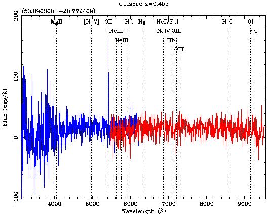
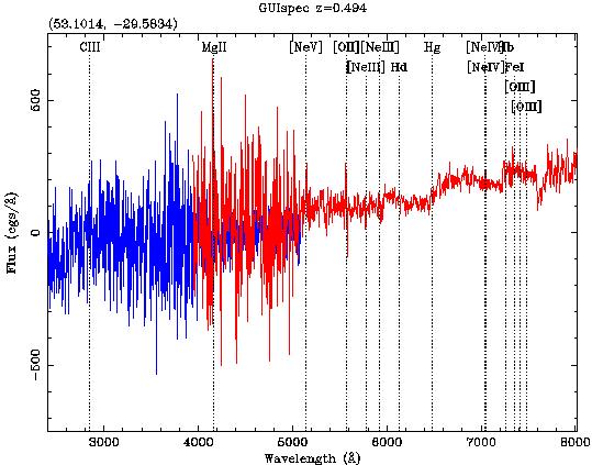
124 Chapter 5: Comparison with SWIRE photometry

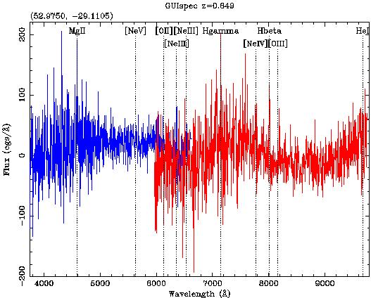
125 Spectra and Object Classes 125

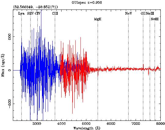
126 Chapter 5: Comparison with SWIRE photometry

127 Spectra and Object Classes Figure 5.7: Spectra with available. and without all [SII], Hα, [OIII], Hβ, [NII] lines Figure 5.7 Shows the spectra of all objects which are not classified as U/HLIRGs and couldn t be used for the emission line diagnostic. With some exceptions, they are noisy spectra or single emission line objects. In this case the line is assigned to [OII] (161). Their comparison with photometric redshifts is rather good which make the assignment of the [OII] lines rather logical. Because of the detection of [OII] as a single emission line we expect that these sources exhibit star forming activity. According to the SED fitting these objects are fitted with a starburst template or in some cases there is no IR - excess. Among them, there are spectra with very good quality enabling us to accurately identify spectral features and derive redshifts. Two out of four sources with z > 2 are objects with clear broad lines. The first of them (z = 2.183) is a faint source (R = 23.48) and has no IR - excess according to the IR SED fitting. The second source (z = 2.197) is fitted by a cirrus template. The strong broad lines imply the presence of a strong AGN. The other two sources from this redshift region have no IR - excess. Six of these spectra have strong Hbeta and [OIII] double lines. Four of these sources present a strong [OII] line. Their spectra imply the presence of star-forming domination in agreement with SED fitting. According to IR SED four sources are fitted with a starburst and the remaining to have no excess. 5.6 Comparison with SWIRE photometric results Photometric redshifts provide an excellent tool for studies of the evolutionary properties of galaxies. Their value against spectroscopic redshifts is clear, especially in the case of faint galaxies, for which spectroscopic observations are difficult or impossible. Moreover, photometric methods can estimate the redshifts faster than spectroscopic methods and can be applied to much fainter magnitudes since the bin sizes are larger. The disadvantage of photometric redshifts is that their present lower 127