Study on Bivariate Normal Distribution

Transcript

1 Florida International University FIU Digital Commons FIU Electronic Theses and Dissertations University Graduate School Study on Bivariate Normal Distribution Yipin Shi Florida International University, DOI: /etd.FI Follow this and additional works at: Recommended Citation Shi, Yipin, "Study on Bivariate Normal Distribution" FIU Electronic Theses and Dissertations This work is brought to you for free and open access by the University Graduate School at FIU Digital Commons. It has been accepted for inclusion in FIU Electronic Theses and Dissertations by an authorized administrator of FIU Digital Commons. For more information, please contact

2 FLORIDA INTERNATIONAL UNIVERSITY Miami, Florida STUDY ON BIVARIATE NORMAL DISTRIBUTION A thesis submitted in partial fulfillment of the requirements for the degree of MASTER OF SCIENCE in STATISTICS by Yipin Shi 2012

3 To: Dean Kenneth Furton College of Arts and Sciences This thesis, written by Yipin Shi, and entitled Study on Bivariate Normal Distribution, having been approved in respect to style and intellectual content, is referred to you for judgment. We have read this thesis and recommend that it be approved. B. M. Golam Kibria Kai Huang, Co-Major Professor Jie Mi, Co-Major Professor Date of Defense: November 9, 2012 The thesis of Yipin Shi is approved. Dean Kenneth Furton College of Arts and Sciences Dean Lakshmi N. Reddi University Graduate School Florida International University, 2012 ii

4 ACKNOWLEDGMENTS This thesis would not have been possible without the guidance and the help of those who, in one way or another, contributed and extended their valuable assistance in the preparation and completion of this study. First and foremost, I would like to express the deepest appreciation to my supervising professor Dr. Jie Mi who helped me all the time in the research and writing of this thesis. I cannot find words to express my gratitude to his patience, motivation, and guidance. He continually and convincingly conveyed a spirit of adventure in regard to teaching, research and scholarship. Without his guidance and persistent help, this thesis would not have been possible. It gives me great pleasure in acknowledging the support and help from Dr. Kai Huang, my co-major professor. He helped tutor me in the more esoteric and ingenious methods necessary to run LATEX and MATLAB and gave useful guidance in how to analyse the data from them. Dr. Huang has offered much advice and insight throughout my work on this thesis study. I sincerely appreciate Dr. B. M. Golam Kibria for his time to serve on my committee. He is always ready to offer help and support whenever I needed them. In addition, I would like to thank all the professors in the Department of Mathematics and Statistics who helped and encouraged me when I went throughout the hurdles in my study. Last but not least, a thank you to my dear friends and classmates, Zeyi, Suisui, and Shihua for their unselfish support. iii

5 ABSTRACT OF THE THESIS STUDY ON BIVARIATE NORMAL DISTRIBUTION by Yipin Shi Florida International University, 2012 Miami, Florida Professor Jie Mi, Co-Major Professor Professor Kai Huang, Co-Major Professor Let X, Y be bivariate normal random vectors which represent the responses as a result of Treatment 1 and Treatment 2. The statistical inference about the bivariate normal distribution parameters involving missing data with both treatment samples is considered. Assuming the correlation coefficient ρ of the bivariate population is known, the MLE of population means and variance ξ, η, and σ 2 are obtained. Inferences about these parameters are presented. Procedures of constructing confidence interval for the difference of population means ξ η and testing hypothesis about ξ η are established. The performances of the new estimators and testing procedure are compared numerically with the method proposed in Looney and Jones 2003 on the basis of extensive Monte Carlo simulation. Simulation studies indicate that the testing power of the method proposed in this thesis study is higher. Keywords: Bivariate Normal Distribution, MLE, MSE, Bias, Testing Power iv

6 TABLE OF CONTENTS CHAPTER PAGE 1 Introduction Maximum Likelihood Estimators of Parameters Moments of the Maximum Likelihood Estimators Limits of Estimators Inferences about ξ, η and ξ η Numerical Study Conclusions REFERENCES v

7 LIST OF TABLES TABLE PAGE 1 Estimation of Treatment Mean ξ Estimation of Variance ξ Estimation of Covariance ξ, η Estimation of Standard Deviation ξ η Estimated Width of 95% Confidence Interval for ξ η Coverage Probability of 95% CI for ξ η vi

8 LIST OF FIGURES FIGURE PAGE 1 MSE ξ n 1 = n 2 = 25, ξ = 5.1, σ = MSE ξ n 1 = n 2 = 35, ξ = 5.5, σ = Var ξ n 1 = n 2 = 25, ξ = 5.1, σ = Var ξ n 1 = n 2 = 35, ξ = 5.5, σ = Cov ξ, η n 1 = n 2 = 5, ξ = 5.1, σ = Cov ξ, η n 1 = n 2 = 35, ξ = 5.5, σ = StDev ξ η n 1 = n 2 = 5, ξ = 5.1, σ = StDev ξ η n 1 = n 2 = 35, ξ = 5.5, σ = Width of 95% CI for ξ η n 1 = n 2 = 5, ξ = 5.1, σ = Width of 95% CI for ξ η n 1 = n 2 = 35, ξ = 5.5, σ = Type I Error n 1 = n 2 = 35, ξ = 5, σ = Testing Power n 1 = n 2 = 35, ξ = 5.3, σ = vii

9 1. Introduction The bivariate normal distribution is one of the most popular distributions used in a variety of fields. Since the bivariate normal PDF has several useful and elegant properties, bivariate normal models are very common in statistics, econometrics, signal processing, feedback control, and many other fields. Let X, Y be bivariate normal random vectors which represent the responses that result from Treatment 1 and Treatment 2. Historically, most of the studies collect paired data. That is, it is assumed that observations are paired and sample consists of n pairs x 1, y 1, x 2, y 2,..., x n, y n. However, in the real world, the available sample data may be incomplete in the sense that measures on one variable X or Y is not available for all individuals in the sample. Such fragmentary data may arise because some of the data are lost e.g., in an archaeological field, or because certain data were purposely not collected. The decision not to measure both variables X and Y simultaneously may be reached because of the cost of measurement, because of limited time, because the measurement of one variable may alter or destroy the individual measured e.g., in mental testing, and so forth. Therefore, either by design, carelessness or accident, the data in a study may consist of a combination of paired correlated and unpaired uncorrelated data. Typically, such data will consist of subsamples of which one has n 1 observations on responses because of Treatment 1 and the other has n 2 observations on responses because of treatment 2 are independent of each other, and another subsample which consists of paired observations taken under both treatments. Statistical inference derived from complete paired data and incomplete unpaired data is one of the important applied problems because of its common occurrence in practice. 1

10 Missing values have been discussed in the literature for modeling bivariate data. Much of the work involved establishing and testing hypothesis about the difference of the population means. Several authors have investigated the problem of estimation and testing the difference of the means in the case of incomplete samples from bivariate normal distributions. Mehta and Gurland 1969a consider the problem of testing the equality of the two means in the special case when the two variances are the same. Morrison 1972, 1973, and Lin and Stivers 1975 have also considered this special case and have provided different test statistics. The problem of estimating the difference of two means has been further investigated by Mehta and Gurland 1969b, Morrison 1971, Lin 1971, and Mehta and Swamy Bhoj 1991a, b tested for the equality of means for bivariate normal data. To make use of all the data and takes into account the correlation between the paired observations, Looney and Jones 2003 compared several methods and proposed the correlated z-test method for analyzing combined samples of correlated and uncorrelated data. In their study, it is assumed that there is another random sample of n 1 subjects exposed to Treatment 1 that is independent of a random sample of n 2 subjects exposed to Treatment 2. Let u 1, u 2,..., u n1 and v 1, v 2,..., v n2 denote the observed values for the independent subjects exposed to Treatment 1 and Treatment 2, respectively. Suppose also that there are n 3 paired observations under treatments 1 and 2. Let x 1, y 1, x 2, y 2,..., x n, y n denote the observed pairs. It is assumed that the x-and u-observations come from a common normal parent population and that the y-and v-observations come from another possibly different common normal parent population. The proposed method is developed using asymptotic results and is evaluated using simulation. The simulation 2

11 results indicate that the proposed method can provide substantial improvement in testing power when compared with the corrected z method of recommended in Looney and Jones In this research, we want to study the bivariate normal model with incomplete data information on both variates. We will derive the maximum likelihood estimators of the distribution parameters, investigate properties such as unbiasedness, and study the asymptotic distribution of these estimators as well. Showing that the asymptotic normality of the estimators, we then will be able to construct confidence intervals of the two population means and their difference, and test hypothesis about these parameters. The performance of our new estimators will be studied after using Monte Carlo simulations, and will be compared with those estimators that existed in the literature. 3

12 2. Maximum Likelihood Estimators of Parameters Let x i, y i, 1 i n be a paired sample from bivariate normal population X Y N ξ η, σ 2 1 ρ ρ 1 where 1 < ρ < 1 is known, but ξ, η, and σ 2 are unknown. In addition, suppose an independent sample {u 1,..., u n1 } on the basis of observations on X, and another independent sample {v 1,..., v n2 } derived from observations on Y is also available. In the present section we should derive the MLEs of ξ, η, and σ 2 derived from data {x i, y i, 1 i n; u j, 1 j n 1 ; v j, 1 j n 2 }. Because of the independence of {X i, Y i, 1 i n}, {U j, 1 j n 1 }, and {V j, 1 j n 2 }, the likelihood equation is n 1 1 Lξ, η, σ = e u j ξ 2σ 2 2πσ n 1 2πσ 2 1 ρ 2 e 2 n2 1 e y i η 2πσ n 1 +n 2 = 2π 2 n 1 ρ 2 n 2 e 1 21 ρ 2 σ n 1+n 2 +2n [ n x i ξ 2 σ ρ 2 [ n 1 e x i ξ 2 σ 2 u j ξ2 2σ 2 2 2σ 2 ] 2ρ x i ξy i η σ 2 + y i η2 σ 2 n 2 v j η2 2σ 2 2ρ n x i ξy i η n y σ 2 + i η 2 ] σ 2 Hence, the log-likelihood function is 4

13 n 1 ln Lξ, η, σ =C n 1 + n 2 + n ln σ 2σ 2 2σ 2 x i ξ 2 2ρ x i ξy i η 1 21 ρ 2 + σ 2 σ 2 u j ξ 2 n 2 v j η 2 y i η 2 σ where C = n 1+n 2 +2n 2 ln 2π n 2 ln1 ρ2 From 2.1 we have ln L ξ = n 1 2 u j ξ 2σ ρ 2 2 x i ξ σ 2 + 2ρ y i η σ 2 = n 1 u j ξ σ ρ 2 x i ξ σ 2 ρ y i η σ ln L η = n 2 v j η σ ρ 2 y i η σ 2 ρ x i ξ σ Setting ln L/ ξ = 0, we obtain from 2.2 that n 1 1 ρ 2 u j ξ + x i ξ ρ y i η = Similarly, by setting ln L/ η = 0 from 2.3, we obtain 5

14 n 2 1 ρ 2 v j η + y i η ρ x i ξ = Note that Equation 2.4 further gives n 1 1 ρ 2 u j n 1 1 ρ 2 ξ + x i nξ ρ y i η = 0 [ n1 1 ρ 2 + n ] n 1 ξ = 1 ρ 2 u j + x i ρ y i η 2.6 In the same way, Equation 2.5 further gives [ n2 1 ρ 2 + n ] n 2 η = 1 ρ 2 v j + y i ρ x i ξ η = n 2 1 ρ 2 v j + y i ρ x i ξ n 2 1 ρ 2 + n. 2.7 Substituting 2.7 into 2.6 yields [ n1 1 ρ 2 + n ] n 1 ξ =1 ρ 2 u j + x i ρ + nρ or n 2 1 ρ 2 v j + y i y i ρ n 2 1 ρ 2 + n x i ξ, [ n1 1 ρ 2 + n ] [ n 2 1 ρ 2 + n ] ξ 6

15 =1 ρ 2 [ n 2 1 ρ 2 + n ] n 1 u j + [ n 2 1 ρ 2 + n ] n x i ρ [ n 2 1 ρ 2 + n ] n [ n 2 + nρ 1 ρ 2 v j + y i ρ ] x i ξ =1 ρ 2 [ n 2 1 ρ 2 + n ] n 1 u j + [ n 2 1 ρ 2 + n ] n x i ρ [ n 2 1 ρ 2 + n ] n n 2 + nρ1 ρ 2 v j + nρ y i nρ 2 x i + n 2 ρ 2 ξ, y i y i {[ n1 1 ρ 2 + n ] [ n 2 1 ρ 2 + n ] n 2 ρ 2} ξ =1 ρ 2 [ n 2 1 ρ 2 + n ] n 1 u j + [ n 2 1 ρ 2 + n nρ 2] n ρ1 ρ 2 n 2 n 2 y i + nρ1 ρ 2 { [n2 =1 ρ 2 1 ρ 2 + n ] n 1 u j + n 2 + n [ ] n 2 + ρ1 ρ 2 n v j n 2 y i v j } x i x i 2.8 Note that [ n1 1 ρ 2 + n ] [ n 2 1 ρ 2 + n ] n 2 ρ 2 =n 1 n 2 1 ρ n 1 n1 ρ 2 + n 2 n1 ρ 2 + n 2 n 2 ρ 2 =1 ρ 2 [ n 1 n 2 1 ρ 2 + n 1 n + n 2 n + n 2] =1 ρ 2 [ n 1 + nn 2 + n n 1 n 2 ρ 2] 2.9 The MLE ξ of ξ can be obtained from 2.8 and 2.9 as 7

16 ξ = [ ] n 1 n 2 [n 2 1 ρ 2 + n] u j + n 2 + n x i + ρ n v j n 2 y i Thus, the MLE η of η can be obtained n 1 + nn 2 + n n 1 n 2 ρ η = [ ] n 2 n 1 [n 1 1 ρ 2 + n] v j + n 1 + n y i + ρ n u j n 1 x i n 1 + nn 2 + n n 1 n 2 ρ To obtain the MLE of σ 2 we differentiate ln Lξ, η, σ with respect to σ 2 and have ln L σ 2 n 1 n 2 u j ξ 2 v j η 2 = n 1 + n 2 + 2n + + 2σ 2 2σ 4 2σ 4 1 x i ξ 2 2ρ x i ξy i η ρ 2 σ 4 σ 4 y i η 2 σ 4 Setting ln L/ σ 2 = 0, we obtain n 1 + n 2 + 2nσ 2 n 1 n 2 = u j ξ 2 + v j η 2 + Therefore, the MLE σ 2 of σ 2 is x i ξ 2 2ρ x i ξy i η + 1 ρ 2 y i η 2 σ 2 = n 1 u j ξ 2 n 2 + n 1 + n 2 + 2n v j η 2 + 8

17 + x i ξ 2 2ρ x i ξ y i η + 1 ρ 2 n 1 + n 2 + 2n y i η Summarizing the above, we have the following results. Theorem 2.1 The MLEs of parameters ξ, η, σ 2 are given by ξ = η = [ n 1 n 2 [n 2 1 ρ 2 + n] u j + n 2 + n x i + ρ n v j n 2 n 1 + nn 2 + n n 1 n 2 ρ 2 [ n 2 n 1 [n 1 1 ρ 2 + n] v j + n 1 + n y i + ρ n u j n 1 n 1 + nn 2 + n n 1 n 2 ρ 2 ] y i ] x i σ 2 = n 1 + u j ξ 2 n 2 + v j η 2 n 1 + n 2 + 2n x i ξ 2 2ρ x i ξ y i η + 1 ρ 2 n 1 + n 2 + 2n y i η 2 9

18 3. Moments of the Maximum Likelihood Estimators We have derived the MLEs of ξ, η, σ 2 in the previous section. Now we will study the properties of these estimators. Theorem 3.1 Both ξ and η are unbiased estimators of ξ and η. The variances of ξ and η are as follows. V ar ξ = σ 2 n1 [n 2 1 ρ 2 + n] 2 + nn 2 + n 2 ρ 2 n 2 nn 2 + n [n 1 + nn 2 + n n 1 n 2 ρ 2 ] 2 λ 2 1σ 2 V ar η = σ 2 n2 [n 1 1 ρ 2 + n] 2 + nn 1 + n 2 ρ 2 n 1 nn 1 + n [n 1 + nn 2 + n n 1 n 2 ρ 2 ] 2 λ 2 2σ 2 Proof. We have E ξ = [n 21 ρ 2 + n] n 1 ξ + n 2 + nnξ + ρ [nn 2 η n 2 nη] n 1 + nn 2 + n n 1 n 2 ρ 2 = n 1n 2 1 ρ 2 ξ + n 1 nξ + n 2 + nnξ n 1 + nn 2 + n n 1 n 2 ρ 2 = n 1n 2 + n 1 n + n 2 n + n 2 n 1 n 2 ρ 2 n 1 + nn 2 + n n 1 n 2 ρ 2 ξ = ξ Similarly, we can show that E η = η. That is, both ξ and η are unbiased estimators of ξ and η. To compute V ar ξ, we observe that [ n1 + nn 2 + n n 1 n 2 ρ 2] 2 V ar ξ = [ n 2 1 ρ 2 + n ] 2 n1 σ 2 + n 2 + n 2 nσ 2 + ρ 2 [ n 2 n 2 σ 2 + n 2 2nσ 2] 10

19 2n 2 + nn 2 ρ Cov X i, Y i =n 1 [ n2 1 ρ 2 + n ] 2 σ 2 + nn 2 + n 2 σ 2 + ρ 2 n 2 nn + n 2 σ 2 2n 2 + nn 2 ρ nρσ 2 =n 1 [ n2 1 ρ 2 + n ] 2 σ 2 + nn 2 + n 2 σ 2 ρ 2 n 2 nn 2 + nσ 2 [ =σ {n 2 1 n2 1 ρ 2 + n ] } 2 + nn2 + n 2 ρ 2 n 2 nn 2 + n, So V ar ξ is exactly the same as claimed in the theorem. The variance of η can be derived in the same manner. Corollary 1 Both ξ and η follow normal distributions, i.e., ξ Nξ, λ 2 1σ 2 and η Nη, λ 2 2σ 2. Corollary 2 ξ, η follows bivariate normal distribution with mean vector ξ, η and covariance matrix Σ = λ2 1σ 2 σ 12 σ 12 λ 2 2σ 2 where σ 12 = ρnσ 2 n 1 +nn 2 +n n 1 n 2 ρ 2 Proof. We need only to derive the covariance between ξ and η. According to Theorem 2.1, we have [ n1 + nn 2 + n n 1 n 2 ρ 2] 2 ξ ξ η η { [n2 = 1 ρ 2 + n ] [ n 1 n 2 U j ξ + n 2 + n X i ξ + ρ n V j η 11

20 ]} { [n1 n 2 Y i η 1 ρ 2 + n ] n 2 V j η + n 1 + n Y i η [ ]} n 1 +ρ n U j ξ n 1 X i ξ 3.1 Because of the assumed independences it follows that [ n1 + nn 2 + n n 1 n 2 ρ 2] 2 Cov ξ, η { [n2 =E 1 ρ 2 + n ] } n 1 n 1 U j ξ ρn U j ξ { } + E n 2 + n X i ξ n 1 + n Y i η { + E n 2 + n X i ξ ρn 1 } X i ξ { n 2 + E ρn V j η [n 1 1 ρ 2 + n ] } n 2 V j η { } + E ρn 2 Y i η n 1 + n Y i η { + E ρn 2 Y i η ρn 1 } X i ξ E 1 + E 2 + E 3 + E 4 + E 5 + E In the following we will derive each E i, 1 i 6. We have E 1 = ρn [ n 2 1 ρ 2 + n ] E { n1 = ρn [ n 2 1 ρ 2 + n ] V ar = ρn [ n 2 1 ρ 2 + n ] n 1 σ 2 } n 1 U j ξ U j ξ n1 U j ξ = ρn 1 n [ n 2 1 ρ 2 + n ] σ 2 ;

21 { E 2 = n 1 + nn 2 + n E X i ξ } Y i η = n 1 + nn 2 + n ncovx 1, Y 1 = n 1 + nn 2 + n nρσ 2 = ρnn 1 + nn 2 + nσ 2 ; 3.4 { } E 3 = ρn 1 n 2 + n E X i ξ X i ξ = ρn 1 n 2 + n V ar = ρn 1 n 2 + n nσ 2 X i ξ = ρn 1 nn 2 + nσ 2 ; 3.5 E 4 = ρn [ n 1 1 ρ 2 + n ] E { n2 = ρn [ n 1 1 ρ 2 + n ] V ar = ρn [ n 1 1 ρ 2 + n ] n 2 σ 2 } n 2 V j η V j η n2 V j η = ρn 2 n [ n 1 1 ρ 2 + n ] σ 2 ; 3.6 { } E 5 = ρn 2 n 1 + n E Y i η Y i η = ρn 2 n 1 + n V ar Y i η 13

22 = ρn 2 n 1 + n nσ 2 = ρn 2 nn 1 + nσ 2 ; 3.7 { E 6 = ρ 2 n 1 n 2 E X i ξ { = ρ 2 n 1 n 2 E } Y i η } X i ξy j η X i ξy i η + i j { } = ρ 2 n 1 n 2 E X i ξy i η + E X i ξy j η i j = ρ 2 n 1 n 2 {ne [X 1 ξy 1 η]} = ρ 2 n 1 n 2 {ncovx 1, Y 1 } = ρ 2 n 1 n 2 nρσ 2 = ρ 3 n 1 n 2 nσ Therefore, from it follows that [ n1 + nn 2 + n ρ 2 n 1 n 2 ] 2 Cov ξ, η =ρn 1 n [ n 2 1 ρ 2 + n ] σ 2 + ρnn 1 + nn 2 + nσ 2 ρn 1 nn 2 + nσ 2 + ρn 2 n [ n 1 1 ρ 2 + n ] σ 2 ρn 2 nn 1 + nσ 2 + ρ 3 n 1 n 2 nσ 2 =ρnσ [ 2 n 1 + nn 2 + n n 1 n 2 ρ 2] and thus 14

23 Cov ξ, η = ρnσ 2 n 1 + nn 2 + n n 1 n 2 ρ 2 λ 12σ Below we will derive the mean of σ 2. To this end, we need to find the following expectations: First, we will derive E E E E n1 U j ξ n2 2, E V j η 2, n1 X i ξ 2, E Y i η 2, and X i ξ Y i η U j ξ 2. Note that ξ ξ [ ] n 1 n 2 [n 2 1 ρ 2 + n] U j + n 2 + n X i + ρ n V j n 2 Y i = ξ n 1 + nn 2 + n n 1 n 2 ρ 2 [ ] n 1 n 2 [n 2 1 ρ 2 + n] U j ξ + n 2 + n X i ξ + ρ n V j n 2 Y i = n 1 + nn 2 + n n 1 n 2 ρ 2 Hence, without loss of generality we can assume ξ = 0 in the following. We thus have E n1 U j ξ 2 15

24 =E =E n1 n1 Uj 2 2 Uj 2 2 ξu j + ξ n 1 2E ξ U j + n 1 V ar ξ n 1 =n 1 σ 2 2E ξ U j + n 1 V ar ξ n1 2 2 [n 2 1 ρ 2 + n] E U j ξ =n 1 σ 2 + n n 1 + nn 2 + n n 1 n 2 ρ 2 1 V ar =n 1 σ 2 2n 1 [n 2 1 ρ 2 + n] σ 2 n 1 + nn 2 + n n 1 n 2 ρ 2 + n 1V ar ξ 3.10 Similarly, it can be shown that E n2 V j η 2 The mean of = n 2 σ 2 2n 2 [n 1 1 ρ 2 + n] σ 2 n 1 + nn 2 + n n 1 n 2 ρ 2 + n 2V ar η 3.11 X i ξ 2 can be obtained as follows: E =E =E X i ξ 2 X 2 i 2 ξx i + ξ 2 X 2 i 2E ξ ξ2 X i + ne 2 n 2 + n E X i n 2 ρ E X i Y i ξ =nσ nv ar n 1 + nn 2 + n n 1 n 2 ρ [ 2 nn 2 + nσ 2 n 2 ρ EX i Y i + ] EX i Y k ξ =nσ 2 i k 2 + nv ar n 1 + nn 2 + n n 1 n 2 ρ 2 =nσ 2 2 nn 2 + nσ 2 n 2 ρ ncovx 1, Y 1 n 1 + nn 2 + n n 1 n 2 ρ 2 + nv ar 16 ξ

25 =nσ 2 [n 2 n1 ρ 2 + n 2 ] σ 2 2 ξ n 1 + nn 2 + n n 1 n 2 ρ + nv ar 2 =nσ 2 2n [n 21 ρ 2 + n] σ 2 n 1 + nn 2 + n n 1 n 2 ρ 2 + nv ar ξ 3.12 In the same manner we can obtain E Y i η 2 = nσ 2 2n [n 11 ρ 2 + n] σ 2 ξ n 1 + nn 2 + n n 1 n 2 ρ + nv ar 2 Now, notice that once again we can assume ξ = η = 0 without loss of generality, and 3.13 Note that X i ξ Y i η = X i Y i ξ Y i η X i + n ξ η 3.14 E X i Y i = nex 1 Y 1 = ncovx 1, Y 1 = nρσ E ξ 2 n 2 + ne X i Y i ρn 2 E Y i Y i = n 1 + nn 2 + n n 1 n 2 ρ 2 n 2 + ne X i Y i ρn 2 V ar Y i = n 1 + nn 2 + n n 1 n 2 ρ 2 = n 2 + nncovx 1, Y 1 ρn 2 nσ 2 n 1 + nn 2 + n n 1 n 2 ρ 2 = n 2 + nnρσ 2 n 2 nρσ 2 n 1 + nn 2 + n n 1 n 2 ρ 2 = n 2 ρσ 2 n 1 + nn 2 + n n 1 n 2 ρ 2, 3.16 E η X i = n 2 ρσ 2 n 1 + nn 2 + n n 1 n 2 ρ 2,

26 and, E ξ η = Cov ξ, η which is given by 3.9. Combining and 3.9, we obtain E =nρσ 2 =nρσ 2 Finally, we have X i ξ Y i η 2n 2 ρσ 2 n 1 + nn 2 + n n 1 n 2 ρ 2 + n ρnσ 2 n 1 + nn 2 + n n 1 n 2 ρ 2 n 2 ρσ 2 n 1 + nn 2 + n n 1 n 2 ρ n 1 + n 2 + 2nE σ 2 =E + { n1 U j ξ n V j η 2 + X i ξ 2 2ρ X i ξy i η + 1 ρ 2 Y i η 2 = [n 1 σ 2 2n 1 [n 2 1 ρ 2 + n] σ 2 ξ ] n 1 + nn 2 + n n 1 n 2 ρ + n 1V ar 2 + [n 2 σ 2 2n ] 2 [n 1 1 ρ 2 + n] σ 2 n 1 + nn 2 + n n 1 n 2 ρ + n 2V ar η 2 {[ + 1 ρ 2 1 nσ 2 2n [n 21 ρ 2 + n] σ 2 ξ ] n 1 + nn 2 + n n 1 n 2 ρ + nv ar 2 + [nσ 2 2n [n ] 11 ρ 2 + n] σ 2 + nv ar η n 1 + nn 2 + n n 1 n 2 ρ2 [ ]} 2ρ nρσ 2 n 2 ρσ 2 n 1 + nn 2 + n n 1 n 2 ρ 2 =n 1 + n 2 σ 2 2n 1 [n 2 1 ρ 2 + n] + 2n 2 [n 1 1 ρ 2 + n] n 1 + nn 2 + n n 1 n 2 ρ 2 σ ρ 2 1 { 2n1 ρ 2 σ 2 2n [n 21 ρ 2 + n] + 2n [n 1 1 ρ 2 + n] 2n 2 ρ 2 n 1 + nn 2 + n n 1 n 2 ρ 2 σ 2 18

27 } +n 1 V ar ξ + n 2 V ar η + nv ar ξ + nv ar η =n 1 + n 2 + 2nσ 2 2n 1 [n 2 1 ρ 2 + n] + 2n 2 [n 1 1 ρ 2 + n] n 1 + nn 2 + n n 1 n 2 ρ 2 σ 2 1 ρ 2 1 2n [n 21 ρ 2 + n + n 1 1 ρ 2 + n nρ 2 ] σ 2 n 1 + nn 2 + n n 1 n 2 ρ 2 [ ] + n 1 V ar ξ + n 2 V ar η + 1 ρ 2 1 n V ar ξ + V ar η 3.19 Summarizing the above, we obtain Theorem 3.2 The mean of σ 2 is E σ 2 = σ 2 n 1 + n 2 + 2n 1 A 1 + A where A 2 = A 1 =n 1 + n 2 + 2nσ 2 2n 1 [n 2 1 ρ 2 + n] + 2n 2 [n 1 1 ρ 2 + n] n 1 + nn 2 + n n 1 n 2 ρ 2 σ 2 1 ρ 2 1 2n [n 21 ρ 2 + n 1 1 ρ 2 + 2n nρ 2 ] σ 2 n 1 + nn 2 + n n 1 n 2 ρ 2 { [ ]} n 1 V ar ξn + n 2 V ar η n + 1 ρ 2 1 n V ar ξn + V ar η n /σ 2, here we denote ξ and η as ξ n and η n to emphasize their dependence on n. Corollary: Suppose that there exist constants 0 α, β < such that lim n n 1 /n = α and lim n n 2 /n = β, then the MLE σ 2 is asymptotically unbiased. Proof. From 3.20 we see that E σ 2 can be expressed as E σ 2 = σ 2 + o1 + [ ] V ar ξn + V ar η n O1 According to Theorem 3.1 it holds thatv ar ξn = o1 and V ar η n = o1. Hence 19

28 E σ 2 = σ 2 + o1 + o1o1 = σ 2 + o1 and E σ 2 σ 2 as n. 20

29 4. Limits of Estimators In Section 2 the MLEs ξ, η and σ 2 are derived. In the present section we will consider the limits of these estimators as sample size goes to infinity. To this end we assume n 1 = n 1 n and n 2 = n 2 n, i.e., both n 1 and n 2 are functions of the number of paired observations. Under this assumption the following result holds. Here, in order to emphasize the dependence of ξ, η and σ 2 on sample size we will denote ξ n = ξ, η n = η, and σ n 2 = σ 2. Theorem 4.1 Suppose n 1 = n 1 n and n 2 = n 2 n and there exist constants α and β such that n 1 /n α < and n 2 /n β < as n. Then the following is true a lim n ξn = ξ, with probability one b lim n η n = η, with probability one c lim n σ n 2 = σ 2, with probability one. That is, all the three estimators ξ, η and σ 2 are strongly consistent. Proof. The MLE ξ n can be rewritten as [ n2 ξ n = n 1 ρ ] n1 n U n1 + n 2 n + 1 X n + ρ [ ] n 2 n V n2 n 2 n Y n n1 n + 1 n 2 n + 1, n 1 n n2 n ρ 2 n 1 n 2 where U n1 = U j /n 1, V n2 = V j /n 2, etc. And so lim ξ n = [β1 ρ2 + 1] αξ + β + 1ξ + ρ [βη βη] n α + 1β + 1 αβρ 2 = [β1 ρ2 + 1] αξ + β + 1ξ α + 1β + 1 αβρ 2 = ξ 21

30 with probability one by the Law of Large Numbers. The result b can be shown in the same way. To prove result c we first note that 1 n X i ξ n 2 = 1 [ ] 2 X i ξ ξ n ξ n { } = 1 X i ξ 2 2 ξ n ξ X i ξ + n ξ n ξ 2 n X i ξ 2 X i ξ = n 2 ξ n ξ n + ξ n ξ 2 and consequently Similarly it can be shown that 1 lim n n X i ξ n 2 = σ 2. lim n 1 1 n 1 n 1 U j ξ n 2 = σ 2, lim n 2 1 n 2 n 2 V j η n 2 = σ 2, As far as 1 lim n n Y i η n 2 = σ 2. X i ξ n Y i η n we have 22

31 1 n X i ξ n Y i η n = 1 [ ] X i ξ ξ n ξ [Y i η η n η] n { = 1 X i ξy i η η n η X i ξ ξ n ξ n } +n ξ n ξ η n η Y i η and thus 1 lim n n X i ξ n Y i η n = CovX, Y = ρσ 2 with probability one, as n. Rewriting σ 2 n as σ 2 n = n 1 n + 1 n 1 n 1 1 ρ 2 1 [ 1 n U j ξ n 2 + n 2 n 1 n + n 2 n n n 2 n 2 X i ξ n 2 2ρ 1 n V j η n 2 X i ξ n Y i η n + 1 n n 1 n + n 2 n + 2 ] Y i η n 2 and letting n, we obtain σ 2 n ασ2 + βσ ρ 2 1 [σ 2 2ρ ρσ 2 + σ 2 ] α + β + 2 =σ 2 α + β + 1 ρ ρ 2 α + β = σ 2

32 with probability one, as n. This ends the proof. 24

33 5. Inferences about ξ, η and ξ η We will consider inferences about ξ and ξ η. The discussion on η is similar and thus is omitted. Theorem 5.1 Suppose that there exist constants 0 α, β < such that n 1 /n α and n 2 /n β as n, then a 1-γ100% approximate confidence interval of ξ can be obtained as ξ ± z γ/2 σ ξ, where σ ξ = λ 2 1 σ 2 = λ 1 σ provided n 1 + n 2 + 2n is sufficiently large. Proof. From Corollary 1 to Theorem 3.1, it is easy to see that ξ follows normal distribution. Also, E ξ = ξ, V ar ξ = λ 2 1σ 2, and ξ Nξ, λ 2 1σ 2. Hence, ξ ξ λ 1 σ N0, 1 Now from ξ ξ λ = σ σ ξ ξ 1 σ λ 1 σ it follows that ξ ξ λ 1 σ N0, 1 in distribution as n due to the Slutsky s Theorem. Therefore, if n then ξ ξ λ 1 σ N0, 1, approximately, which yields the desired result immediately. 25

34 In practice, one is more often interested in the difference ξ η. In this regard, we have the following result. Theorem 5.2 Under the same assumption in Theorem 5.1, a 1 γ approximate confidence interval is given by ξ η ± z γ/2 σ ξ η where σ ξ η is defined by 5.1 and 5.2 below. Proof. Obviously ξ η is a normal random variable with mean ξ η. The variance of ξ η is σ 2 ξ η V ar ξ η = V ar ξ + V ar η 2Cov ξ, η 5.1 where V ar ξ and V ar η are derived in Theorem 3.1, and Cov ξ, η is given by 3.9. The estimator of σ 2 ξ η is obtained from replacing σ 2 by σ 2 in the expression of σ 2 ξ η, i.e., σ 2 ξ η = σ 2 ξ η σ 2 = σ The rest of the proof is then the same as Theorem

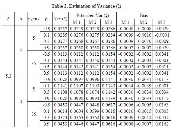
35 6. Numerical Analysis A MATLAB simulation is carried out in order to analyze the performance of the estimators with incomplete observations. With η=5, paired sample size n=30 and N =10000 replications, combinations of different levels of unpaired sample size n 1 =n 2 =5, 25 and 35, ξ=5, 5.1, 5.3 and 5.5, σ=1 and 2, and ρ=-0.9,...,0.9 are used to estimate the Treatment Mean, Variance, Covariance, Standard Deviation, 95% Confidence Interval, Coverage Probability, Type I Error, and Testing Power. The calculated results with known ρ referred to as Method 1 hereafter, legend red circle in Figures and estimated ρ refered to as Method 2 hereafter, legend green cross in the Figures are compared with the results calculated with the method proposed by Looney and Jones 2003referred to as Method 3 hereafter, legend blue diamond in the Figures From the tables and figures, we can see that the results by Method 1 and Method 2 are quite close. Comparing the new Methods with Method 3, we have observations as: a Treatment Mean ξ of Component X Table 1, Figure 1 & 2: The MSEs of the estimators by the new Methods are smaller than those by Method 3, and so the new Methods estimate the treatment mean better. The M SEs of the estimators by the new Methods are smaller than those by Method 3.. The MSEs of the estimators increase when σ increase, decrease when unpaired sample size increase, do not change with treatment means. b Variance of ξ and η Table 2, Figure 3 & 4: V ar ξ and V ar η increase when σ increase, decrease when the number of unpaired observations increase, do not change with treatment means. The V ARs of the estimators by the new Methods are smaller than those by Method 3. 27

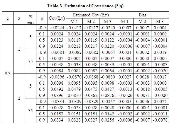
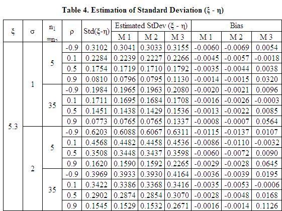
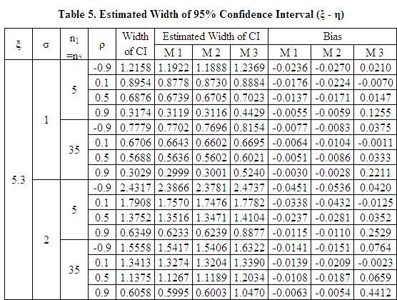
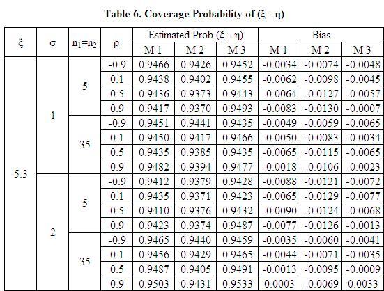
36 c Covariance of ξ, η Table 3, Figure 5 & 6: Cov ξ, η increase when σ and ρ increase; the slopes become smaller when sample size of unpaired observations get larger. All three methods have similar values. d Standard Deviation of ξ η Table 4, Figure 7 & 8: StDev ξ η increase when σ increase, decrease when ρ and unpaired sample size increase. In most cases, estimators from the new Methods are less variable than that from Method 3. e 95% Confidence Interval of ξ η Table 5, Figure 9 & 10: Width of 95% CI for ξ η increase when σ increase, decrease when ρ and unpaired sample size increase. In most cases, Method 3 has higher variability than the new Methods. These observations are consistent with those from d, so these provide further evidence to indicate that estimation from the new Methods has less variability than that from Method 3. f Coverage Probability of 95% CI for ξ η Table 6: The Coverage Probability of all three estimators are lower than the nominal 95%. The new Methods coverage probability is slightly lower than that of Method 3. This is the consequence of the observations from part d and e. g Type I Error Figure 11: Type I Error of the three methods are comparable, while the new Methods Type I Error is a little higher. Again, this is because of the observations from d and e. h Testing Power Figure 12: The testing power increase when ρ, ξ η, and unpaired sample size increase; the testing power decrease when σ increase. The new Methods have higher testing power than Method 3 in all cases. 28

37 29

38 30

39 31

40 Figure 1: MSE ξ n 1 = n 2 = 25, ξ = 5.1, σ = 2 Figure 2: MSE ξ n 1 = n 2 = 35, ξ = 5.5, σ = 2 32

41 Figure 3: Var ξ n 1 = n 2 = 25, ξ = 5.1, σ = 2 Figure 4: Var ξ n 1 = n 2 = 35, ξ = 5.5, σ = 2 33

42 Figure 5: Cov ξ, η n 1 = n 2 = 5, ξ = 5.1, σ = 2 Figure 6: Cov ξ, η n 1 = n 2 = 35, ξ = 5.5, σ = 2 34

43 Figure 7: StDev ξ η n 1 = n 2 = 5, ξ = 5.1, σ = 2 Figure 8: StDev ξ η n 1 = n 2 = 35, ξ = 5.5, σ = 2 35

44 Figure 9: Width of 95% CI for ξ η n 1 = n 2 = 5, ξ = 5.1, σ = 2 Figure 10: Width of 95% CI for ξ η n 1 = n 2 = 35, ξ = 5.5, σ = 2 36

45 Figure 11: Type I Error n 1 = n 2 = 35, ξ = 5, σ = 2 Figure 12: Testing Power n 1 = n 2 = 35, ξ = 5.3, σ = 1 37

46 7. Conclusions On the basis of the analytical and numerical results obtained above, we can make a conclusion that with more unpaired observations the bivariate model provide better estimation of the parameters, which indicate that the estimators with incomplete data are more efficient. After comparing with the method proposed by Looney and Jones 2003, the new Methods have higher testing power and better estimation of the distribution parameters. Therefore, it is recommended that we keep the unpaired data in the analysis procedure and use the model established above to obtain better estimation. 38

47 References [1] Anderson, T. W., Maximum likelihood estimates for a multivariate normal distribution when some observations are missing. J. Amer. Statist. Assoc [2] Bhoj, D.S., 1991a. Testing equality of means in the presence of correlation and missing data. Biometrical J. 33, [3] Bhoj, D.S., 1991b. Testing equality of correlated means in the presence of unequal variances and missing values. Biometrical J. 33, [4] Dahiya R.C. and Korwar R.M., Maximum likelihood estimates for a bivariate normal distribution with missing data. The Annals of Statistics, Vol. 8, No. 3, [5] Garren, S.T., Maximum likelihood estimation of the correlation coefficient in a bivariate normal model with missing data. Statistics & Probability Letters, 38, [6] Hartley, H. O. and Hocking, R. R The analysis of incomplete data. Biometrics, 27, [7] Hocking, R. R. and Smith, W. B Estimation of parameters in the multivariate normal distribution with missing observations. J. Amer. Statist. Ass., 63, [8] Lin, Pi-ERH Estimation procedures for difference of means with missing data. J. Amer. Statist. Assoc [9] Lin, Pi-Erh And Stivrs, L. E Testing for equality of means with incomplete data on one variable: A Monte Carlo study. J. Amer. Statist. Assoc [10] Looney, S.W. and Jones P.W., A method for comparing two normal means using combined samples of correlated and uncorrelated data. Statistics in Medicine 22: [11] Mehta, J. S. and Guirland, J. 1969a. Testing equality of means in the presence of correlation. Biometrika [12] Mehta, J. S. and Gurland, J. 1969b. Some properties and an application of a statistic arising in testing correlation. Ann. Math. Statist [13] Mehta, J. S. and Swamy, P. A. V. B Bayesian analysis of a bivariate normal distribution with incomplete observations. J. Amer. Statist. Assoc [14] Morrison, D. F Expectations and variances of maximum likelihood estimates of the multivariate normal distribution parameters with missing data. J. Amer. Statist. Ass., 66,

48 [15] Morrison, D. F The analysis of a single sample of repeated measurements. Biometrics [16] Morrison, D. F A test for equality of means of correlated variates with missing data of one response. Biometrika [17] Wilks, S. S Moments and distributions of estimates of population parameters from fragmentary samples. Ann. Math. Statist., 3,