Phase-Field Variational Implicit Solvation

Transcript

1 Phase-Field Variational Implicit Solvation Bo Li Department of Mathematics and Quantitative Biology Graduate Program UC San Diego KI-Net Conference: Mean-Field Modeling and Multiscale Methods for Complex Physical and Biological Systems UC Santa-Barbara October 31 November 3, 2016

2 Collaborators Modeling and Computation J. Andrew McCammon (UC San Diego) Joachim Dzubiella (Helmholtz Institute, Berlin) Jianwei Che (Parallel Computing Labs, San Diego) Zuojun Guo (Plexxikon, Inc., Berkeley) Li-Tien Cheng (UC San Diego) Shenggao Zhou (Soochow University) Yanxiang Zhao (George Washington University) Hui Sun (UC San Diego & Cal State, Long Beach) Jiayi Wen (Yahoo) Analysis Yanxiang Zhao (George Washington University) Yuan Liu (Fudan University) Shibin Dai (New Mexico State University) Jianfeng Lu (Duke University) Funding: NIH and NSF

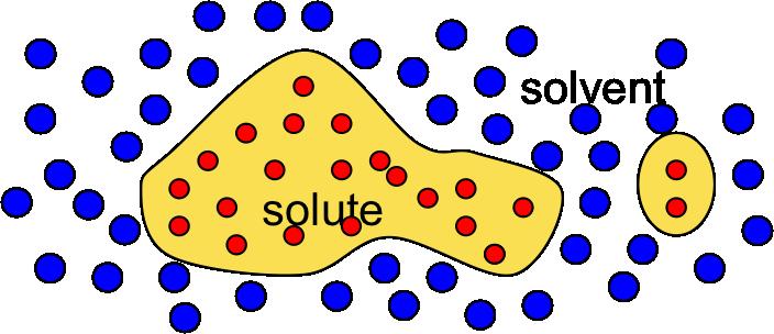
3 Solvation Molecular Modeling: Explicit Solvent vs. Implicit Solvent

4 Dielectric Boundary Based Implicit-Solvent Models Fixed-surface models solvent excluded surface (SES) probing ball vdw surface solvent accessible surface (SAS) G total = G surf + G ele-pb/gb decoupling fitting parameters cavities curvature correction Hasted, Ritson, & Collie, JCP 1948.

5 OUTLINE 1. A Variational Model of Biomolecules 2. The Poisson Boltzmann Electrostatics 3. Convergence of Free Energy 4. Convergence of Force 5. Convergence of Interface

6 1. A Variational Model of Biomolecules Free-energy functional (Dzubiella, Swanson, & McCammon, 2006) F [Γ] = P 0 Vol ( p ) + γ 0 Area (Γ) + ρ 0 U vdw dx + F ele [Γ] w [ F ele [Γ] = ε ] Γ 2 ψ Γ 2 + ρψ Γ χ w B(ψ Γ ) dx U vdw (x) = N i=1 U(i) LJ ( x x i ) U (i) LJ (r) = 4ε i [(σ i /r) 12 (σ i /r) 6] ε Γ ψ Γ χ w B (ψ Γ ) = ρ ψ Γ = ψ on B(s) = k B T M j=1 c j in ( ) e q j s/(k B T ) 1 dielectric boundary w Note: min B = B(0) = 0, B > 0, and B(± ) =. n p Γ ε p=1 ε w=80 xi Q i

7 Free-energy functional F [Γ] = P 0 Vol ( p ) + γ 0 Area (Γ) + ρ 0 w U vdw dx + F ele [Γ] Boundary force F n : Γ R F n = δ Γ F [Γ] = P 0 2γ 0 H + ρ 0 U vdw δ Γ F ele [Γ] δ Γ F ele [Γ] = 1 2 ( 1 1 ) ε Γ ψ Γ n 2 ε p ε w (ε w ε p ) (I n n) ψ Γ 2 + B(ψ Γ ) In particular, δ Γ F ele [Γ] < 0, since ε w > ε p. (Li, Cheng, & Zhang, SIAP 2011) dielectric boundary w n p Γ ε p=1 ε w=80 xi Q i

8 pmf G (kb tot T) PS Tight 100 PS Loose 120 PB Tight PB Loose d (Å)

9 χ A Phase-field model of interface uɛ 1 0 The van der Waals Cahn Hilliard functional [ ξ E ξ [φ] = 2 φ ] ξ W (φ) dx W (φ) = 18φ 2 (φ 1) 2 Why phase-field modeling? An alternative numerical method of implementation. Proof of existence of a minimizer for the sharp-interface free-energy functional. Connection to the Lum Chandler Weeks (LCW) theory of solvation (J. Phys. Chem. B 1999). Description of both bulk and interfacial fluctuations.

10 Phase field φ : w = {φ 0}, p = {φ 1}, and Γ = {φ 1/2}; Dielectric coefficient ε = ε(φ) C 1 (R): ε(φ) = { εw if φ 0 ε p if φ 1 and ε (φ) > 0 if 0 < φ < 1. Phase-field free-energy functional F ξ [φ] = P 0 φ 2 dx + γ 0 [ ξ 2 φ ] ξ W (φ) dx + ρ 0 (φ 1) 2 U vdw dx + F ele [φ] [ F ele [φ] = ε(φ) ] 2 ψ φ 2 + ρψ φ (φ 1) 2 B(ψ φ ) dx ε(φ) ψ φ (φ 1) 2 B (ψ φ ) = ρ ψ φ = ψ on in

11 2. The Poisson Boltzmann Electrostatics F ele [φ] = [ ε(φ) ] 2 ψ φ 2 + ρψ φ (φ 1) 2 B(ψ φ ) dx ε(φ) ψ φ (φ 1) 2 B (ψ φ ) = ρ in (1) ψ φ = ψ on (2) Define A = { u H 1 () : u = ψ on }, [ ] ε(φ) E φ [u] = 2 u 2 ρu + (φ 1) 2 B(u) dx. Theorem 1. For any φ L 4 (), there exists a unique weak solution ψ φ A to (1) and (2) with ψ φ L () C. Moreover, F ele [φ] = E φ [ψ φ ] = min u A E φ[u].

12 Proof. Direct methods in the calculus of variations and standard regularity theory. Key: the L -bound. [ ε Let u = argmin H 1 0 () I [ ], where I [v] = 2 v 2 + B(v)] dx. Let λ > 0 with B (λ) > 1 and B ( λ) < 1. Define λ if u(x) < λ, u λ (x) = u(x) if u(x) λ, λ if u(x) > λ. Then I [u λ ] I [u] and u λ u a.e.. By the convexity of B, 0 χ {u>λ} [B(u) B(λ)] dx + χ {u< λ} [B(u) B( λ)] dx χ {u>λ} B (λ)(u λ) dx + χ {u< λ} B ( λ)(u + λ) dx = χ { u >λ} u λ dx 0. This implies that u λ a.e.. Q.E.D.

13 Theorem 2. Assume sup k 1 φ k L 4 () <, φ k φ in L 1 (), ψ φk = argmin A E φk [ ] (k = 1, 2,... ), and ψ φ = argmin A E φ [ ]. Then ψ φk ψ φ in H 1 () and E φk [ψ φk ] E φ [ψ φ ]. Proof. It suffices to show that any subsequence of {ψ φk } has a further subsequence that converges to ψ φ in H 1 (). With bounds, {ψ φk } has a subsequence that converges to ˆψ weakly in H 1 (), strongly in L 2 (), and a.e. in. Then ˆψ = ψ φ. Further, use the weak formulations for ψ φk and ψ φ to show that ψ φk ψ φ in H 1 () and E φk [ψ φk ] E φ [ψ φ ]. Q.E.D.

14 Now consider the dielectric boundary force. [ F ele [φ] = ε(φ) ] 2 ψ φ 2 + ρψ φ (φ 1) 2 B(ψ φ ) dx ε(φ) ψ φ (φ 1) 2 B (ψ φ ) = ρ ψ φ = ψ on in Heuristics: use δφ as the test function in the weak form of PBE. [ δ φ F ele [φ]δφ = ε (φ) 2 δφ ψ φ 2 ε(φ) ψ φ δ φ ψ φ + ρδ φ ψ φ Hence, 2(φ 1)δφB(ψ φ ) (φ 1) 2 B (ψ φ )δ φ ψ φ ]dx [ ] = ε (φ) 2 ψ φ 2 2(φ 1)B(ψ φ ) δφ dx. δ φ F ele [φ] = ε (φ) 2 ψ φ 2 2(φ 1)B(ψ φ ).

15 Define for any φ L 4 () [ ] 1 f ele (φ) = 2 ε (φ) ψ φ 2 + 2(φ 1)B(ψ φ ) φ, [ ] ε(φ) T ele (φ) = ε(φ) ψ φ ψ φ 2 ψ φ 2 + (φ 1) 2 B(ψ φ ) I. If φ W 1, (), then we have by direct calculations that f ele (φ) = T ele (φ) + ρ ψ φ. If G is open, G, and G C 2 with unit outer normal ν, then we define [ f 0,ele [ G] = 1 ( 1 1 ) ε(χ G ) ψ χg ν 2 2 ε p ε w 1 ] 2 (ε w ε p ) (I ν ν) ψ χg 2 B(ψ χg ) ν.

16 Lemma. If φ W 1, and V Cc 1 (, R 3 ), then f ele (φ) V dx = [T ele (φ) : V ρ ψ φ V ] dx. If φ = χ G with G open, G, C 2, then [ f 0,ele [ G] V ds = Tele (χ G ) : V ρ ψ χg V ] dx. Proof. By direct calculations using the fact that ψ φ is the solution to the BVP of PBE. In particular, for φ = χ G, ε p ψ χg = ρ in G, ε w ψ χg + B (ψ) = ρ in G c, ψ χg G = ψ χg G c ε p ψ χg G ν = ε w ψ χg G c ν Moreover, notice that on G, on G. ψ χg = ( ψ χg ν)ν + (I ν ν) ψ χg on G. Q.E.D.

17 Theorem 3. If sup k 1 φ k L 4 () < and φ k φ a.e., then [ Tele (φ k ) : V ρ ψ φk V ] dx lim k = [ Tele (φ) : V ρ ψ φ V ] dx V C 1 c (, R 3 ). Proof. The key step is to prove ε(φ k ) ψ φk ψ φk dx = lim k Notice that, with ψ k = ψ φk and ψ = ψ φ, ε(φ) ψ φ ψ φ dx. ε(φ k ) ψ k ψ k = ε(φ k ) [( ψ k ψ) ( ψ k ψ) + ψ ( ψ k ψ) + ( ψ k ψ) ψ + ψ ψ]. The result follows from ψ φk ψ φ in H 1 (), φ k φ a.e. in, and the Lebesgue Dominated Convergence Theorem. Q.E.D.

18 Define 3. Convergence of Free Energy F 0 [φ] = P 0 A + γ 0 P (A) + ρ 0 \A U vdw dx + F ele [φ]. Theorem 4. Let ξ k 0. Then Γ-lim k F ξk = F 0 with respect to L 1 ()-convergence. (1) The liminf condition. If φ k φ in L 1 () then lim inf k F ξ k [φ k ] F 0 [φ]. (2) The recovering sequence. For any φ L 1 (φ), there exist φ k L 1 () (k = 1, 2,... ) such that φ k φ in L 1 () and lim sup F ξk [φ k ] F 0 [φ]. k Corollary. There exists G with P (G) < such that F 0 [χ G ] = min φ L 1 () F 0 [φ], which is finite.

19 Proof of Theorem 4. (1) Assume φ k φ a.e. in and {F ξk [φ k ]} converges. Then, [ ξk 2 φ k ] W (φ k ) dx <. ξ k sup k 1 Hence, φ = χ G and φ k χ G in L 2 (). Note that η k (x) := φk (x) 0 2W (t) dt χg a.e., η k = 2W (φ k ) φ k, and sup k 1 η k W 1,1 () <. Hence, P (G) lim inf η k dx k = lim inf 2W (φk ) φ k dx k lim inf k [ ξk 2 φ k ] W (φ k ) dx. ξ k

20 (2) Assume F 0 [φ] <. So, φ = χ G BV () with G. Step 1. Assume G = D with D open, D in C, D in C 2, and H 2 ( D ) = 0. There exist φ k H 1 () such that 0 φ k χ G in, φ k = 1 in G k := {x G : dist(x, G) } ξ k, φ k = 0 in \ G, φ k χ G strongly in L 1 () and a.e. in, [ ξk lim sup k 2 φ k ] W (φ k ) dx P (G). ξ k There exist r 0 > 0 such that N i=1 B(x i, r 0 ) G k G for all k 1. {φ k } is a recovering sequence.

21 Step 2. Assume φ = χ G with 0 < G < and P (G) <. Choose σ k 0 such that B(σ k ) := N i=1 B(x i, σ k ), U 0 on B(σ k ), and 0 < G B(σ k ) < for all k 1. Set Ĝ k = G B(σ k ). Then Ĝk+1 Ĝk and χĝk χ G in L 1 (). So, lim sup F 0 [χĝk ] F 0 [χ G ]. k Fix k 1. There exist open D k,j R 3 (j = 1, 2,... ) satisfying: G k,j := D k,j B(σ k /2); D k,j is C, D k,j is C 2, and H 2 ( D k,j ) = 0; G k,j Ĝk 0; Then lim j F 0[χ Gk,j ] = F 0 [χĝk ], k = 1, 2,...

22 There exist H k = G k,jk such that for all k = 1, 2,... χ Hk χĝk L 1 () < 1/k and F 0 [χ Hk ] F 0 [χĝk ] < 1/k. Since χĝk χ G in L 1 (), we further have lim χ H k χ G L k 1 () = 0 and lim sup F 0 [χ Hk ] F 0 [χ G ]. k By Step 1, we can find for each k 1 a recovering sequence {φ k,l } l=1 for χ H k. Finally, a subsequence {φ k,lk } is a recovering sequence for χ G. Q.E.D.

23 Theorem 5. If φ k χ G a.e., and F ξk [φ k ] F 0 [χ G ] R, then lim φ 2 kdx = G, k [ ξk lim k 2 φ k ] W (φ k ) dx = P (G), ξ k (φ k 1) 2 U vdw dx = U vdw dx, lim k \G lim F ele[φ k ] = F ele [χ G ]. k Proof. We have lim k a k = a and lim k b k = b, provided that lim (a k+b k ) = a+b, lim inf a k a 0 and lim inf b k b 0. k k k We have also that [ ξk lim inf k 2 φ k ] W (φ k ) dx P (G), ξ k lim inf (φ k 1) 2 U vdw dx χ \G U vdw dx. Q.E.D. k {U vdw >0} {U vdw >0}

24 Phase-field forces 4. Convergence of Force f vol (φ) = 2P 0 φ φ, f ξ,sur (φ) = γ 0 [ ξ φ + 1 ] ξ W (φ) φ, f vdw (φ) = 2ρ 0 (φ 1)U vdw φ, in \ {x 1,..., x N } [ ] f ele (φ) = ε (φ) 2 ψ φ 2 2(φ 1)B(ψ φ ) φ. Phase-field stresses T vol (φ) = P 0 φ 2 I, {[ ξ T ξ,sur (φ) = γ 0 2 φ ] } ξ W (φ) I ξ φ φ, T vdw (φ) = ρ 0 (φ 1) 2 U vdw I, T ele (φ) = ε(φ) ψ φ ψ φ [ ] ε(φ) 2 ψ φ 2 + (φ 1) 2 B(ψ φ ) I.

25 Lemma. We have for almost all points in that f vol (φ) = T vol (φ) if φ H 1 (), f ξ,sur (φ) = T ξ,sur (φ) if φ H 2 (), f vdw (φ) = T vdw (φ) ρ 0 (φ 1) 2 U vdw if φ H 1 (), f ele (φ) = T ele (φ) + ρ ψ φ if φ W 1, (). Moreover, we have for any V Cc 1 (, R 3 ) that f vol (φ) V dx = T vol (φ) : V dx if φ H 1 (), f ξ,sur (φ) V dx = T ξ,sur (φ) : V dx if φ H 2 (), [ f vdw (φ) V dx = TvdW (φ) : V + ρ 0 (φ 1) 2 U vdw V ] dx if {x 1,..., x N } supp (V ) = and φ H 1 (), f ele (φ) V dx = [T ele (φ) : V ρ ψ φ V ] dx if φ W 1, ().

26 Sharp-interface forces: Let G be open with G, G in C 2, x i G (i = 1,..., N), and ν the unit outer normal of G. Define f 0,vol [ G] = P 0 ν, f 0,sur [ G] = 2γ 0 Hν, f 0,vdW [ G] = ρ 0 U vdw ν, [ f 0,ele [ G] = 1 2 ( 1 ε p 1 ε w ) ε(χ G ) ψ χg ν 2 1 ] 2 (ε w ε p ) (I ν ν) ψ χg 2 B(ψ χg ) ν.

27 Lemma. We have for any V Cc 1 (, R 3 ) that f 0,vol [ G] V ds = T vol (χ G ) : V dx, G f 0,sur [ G] V ds = γ 0 (I ν ν) : V ds, G G f 0,vdW [ G] V ds = [T vdw (χ G ) : V G G +ρ 0 (1 χ G ) 2 U vdw V ] dx if {x 1,..., x N } supp (V ) =, f 0,ele [ G] V ds = [T ele (χ G ) : V ρ ψ χg V ] dx.

28 Theorem 6. Let G, P (G) <, F 0 [χ G ] is finite, φ k χ G a.e. in, and F ξk [φ k ] F 0 [χ G ]. Then, for any V Cc 1 (, R 3 ), lim T vol (φ k ) : V dx = T vol (χ G ) : V dx, k lim T ξk,sur(φ k ) : V dx = γ 0 (I ν ν) : V dh 2, k G [ (TvdW (φ k ) : V + ρ 0 (φ k 1) 2 U vdw V ] dx lim k = [ TvdW (χ G ) : V + ρ 0 (χ G 1) 2 U vdw V ] dx if {x 1,..., x N } supp (V ) =, lim [T ele (φ k ) : V ρ ψ φk V ] dx k = [T ele (χ G ) : V ρ ψ χg V ] dx. Proof. Each component of energy converges. Then, the key is the convergence of the surface energy. Q.E.D.

29 Force convergence for the van der Waals Cahn Hilliard functional. Theorem 7. Let R n be bounded and open. Let G, P (G) <, φ k χ G a.e. in, and [ ξk lim k 2 φ k ] W (φ k ) dx = P (G). ξ k Then we have for any Ψ C c (, R n n ) that T ξk (φ k ) : Ψ dx = (I ν ν) : Ψ dh n 1. lim k If, in addition, all φ k W 2,2 (), G is open, and G is of C 2, then [ lim ξ k φ k + 1 ] W (φ k ) φ k V dx k ξ k = (n 1) Hν V ds V Cc 1 (, R n ). G G

30 Remark. Energy convergence is necessary. Proof. Asymptotic equipartition of energy: lim k lim k 2 ξk 2 φ W (φ k ) k dx = 0, ξ k k ξ 2 φ k 2 1 W (φ k ) ξ k dx = 0. Need only to prove that for any Ψ C c (, R n n ) T ξk (φ k ) : Ψ dx = (I ν ν) : Ψ dh n 1. lim k G

31 If suffices to prove that for any Ψ C c (, R n n ) ξ k φ k φ k : Ψ dx = ν ν : Ψ dh n 1. lim k G Assume this is true. Notice for any a R n that a 2 = a a : I. Then (I : Ψ)I C c (, R n n ). Hence, [ ξk lim k 2 φ k ] W (φ k ) I : Ψ dx ξ k = lim ξ k φ k 2 I : Ψ dx k = lim ξ k φ k φ k : (I : Ψ)I dx k = ν ν : (I : Ψ)I dh n 1 G = I : Ψ dh n 1. G

32 Fix Ψ C c (, R n n ) and prove now ξ k φ k φ k : Ψ dx = lim k G ν ν : Ψ dh n 1. Let σ > 0. Recall that G = ( j=1 K j) Q, where K j s are disjoint compact sets, each being a subset of a C 1 -hypersurface S j, and Q G with G (Q) = 0. Moreover, j=1 Hn 1 (K j ) = H n 1 ( G) = G () = P (G) <. Choose J so that j=j+1 Hn 1 (K j ) < σ. Choose open U j such that K j U j U j (j = 1,..., J). For each j, we define d j : U j R to be the signed distance to S j, and zero-extend d j to \ U j. Choose ζ j Cc 1 () be such that 0 ζ j 1 on, ζ j = 1 in a neighborhood of K j, supp (ζ j ) U j, and ζ j d j C c (, R n ). Define ν J : R n by ν J = J j=1 ζ j d j. Note that ν j C c (, R n ), ν j 1 on, and ν j = ν on each K j (1 j J).

33 We rewrite ξ k φ k φ k as ( ξ k φ k φ k = ξk φ k + ) ξ k φ k ν J ξ k φ k ( 2W (φ k ) + ) ξ k φ k ν J ξ k φ k ξ k ν J 2W (φ k ) φ k. Finally, lim sup ξ k φ k φ k : Ψ dx ν ν : Ψ dh n 1 k G ( 4σ sup ) L ξ k φ k Ψ L 2 () () + 2σ Ψ L (). k 1 This completes the proof. Q.E.D.

34 5. Convergence of Interface Matched asymptotic analysis of the relaxation dynamics t φ = δ φ F ξ [φ] : t φ = 2P 0 φ + γ 0 [ξ φ 1 ] ξ W (φ) 2ρ 0 (φ 1)U vdw ε (φ) ψ φ 2 + 2(φ 1)B(ψ φ ), ε(φ) ψ φ (φ 1) 2 B (ψ φ ) = ρ, φ = 0 ψ = ψ on, on. Fast time scale. Instantaneous electrostatic relaxation. Perturb the unstable equilibrium φ 0 (x) = 1/2 of t φ = ξ φ 1 ξ W (φ) The most unstable mode is k c = 0. The fastest growth rate is ω(k c ) = O(1/ξ). So, the fast time scale is T = t/ξ.

35 Fast time scale. Assume T = t/ξ and φ(x, t) = φ 0 (x, T ) + ξφ 1 (x, T ) + ξ 2 φ 2 (x, T ) +, ψ(x, t) = ψ 0 (x, T ) + ξψ 1 (x, T ) + ξ 2 ψ 2 (x, T ) +, φ i = 0 (i 0), ψ 0 = ψ, and ψ i = 0 (i 1) on. Plug these into the governing equations and group terms with the same order of ξ to get T φ 0 = γ 0 W (φ 0 ) : x, φ 0 (x, T ) 0 or 1 exponentially as T, ε(φ 0 ) ψ 0 (φ 0 1) 2 B (ψ 0 ) = ρ. Conclusion: Quickly, the system is partitioned into two regions of different dielectric coefficient, and the electrostatics is relaxed.

36 Regular time scale. Assume φ(x, t) = φ 0 (x, t) + ξφ 1 (x, t) + ξ 2 φ 2 (x, t) +, ψ(x, t) = ψ 0 (x, t) + ξψ 1 (x, t) + ξ 2 ψ 2 (x, t) +, φ i = 0 (i 0), ψ 0 = ψ, and ψ i = 0 (i 1) on. Leading order equations W (φ 0 ) = 0, t φ 0 = 2P 0 φ 0 γ 0 W (φ 0 )φ 1 2ρ 0 (φ 0 1)U vdw ε (φ 0 ) ψ (φ 0 1)B(ψ 0 ), ε(φ 0 ) ψ 0 (φ 0 1) 2 B (ψ 0 ) = ρ. Consequences: (1) φ 0 = 0 or 1; (2) {φ 0 = 0} by the BC; and (3) {φ 0 = 1} by the property of U vdw and second equation. Conclusion: These expansions do not hold in the entire region.

37 Assumptions The entire region is the union of an outer and inner region. The outer region is the union of + ξ (t) := {φ(x, t) 1} and (t) := {φ(x, t) 0}. ξ The inner region is a thin layer of width O(ξ) that centers around Γ ξ (t) = {x : φ(x, t) = 1/2} enclosing + ξ (t). This interface is O(ξ)-close to a smooth interface Γ(t) that is independent of ξ. The inner and outer solutions match asymptotically.

38 Local coordinates for a point x in the inter region: x = Φ(y, t) + ξz(t)n(y, t). Φ(, t) : Q(t) Γ ξ (t) a smooth, principal-curvature parameterization, and Q(t) R 3 is an O(ξ)-neighborhood of Γ ξ (t) and Γ(t). z(t) = s(x, t)/ξ with s(x, t) = ±dist (x, Γ ξ (t)). n(y, t) = x s(x, t) is the unit normal to Γ ξ (t) at Φ(y, t). The normal velocity is v(y, t) = t Φ(y, t) n(y, t). The mean curvature is H(y, t) = y n(y, t)/2.

39 Assume the inner expansions φ(x, t) = φ 0 (z, y, t) + ξ φ 1 (z, y, t) + ξ 2 φ2 (z, y, t) +, ψ(x, t) = ψ 0 (z, y, t) + ξ ψ 1 (z, y, t) + ξ 2 ψ2 (z, y, t) +. Leading order equations: z ψ 0 = 0 and v z φ 0 = γ 0 [ zz 2 φ ] 0 W ( φ 0 ). Matching conditions: φ 0 ( ) = 1, φ 0 ( ) = 0, and z φ 0 (± ) = 0. Hence ( ) [ ] 2 1 v z φ 0 dz = γ0 2 ( z φ z= 0 ) 2 W ( φ 0 ) = 0. z= Therefore v = 0. Conclusion: To the leading order, the interface does not move at this time scale.

40 Slow time scale: τ = ξt. Outer expansions W (φ 0 ) = 0, Use the local coordinate ε(φ 0 ) ψ 0 (φ 0 1) 2 B (ψ 0 ) = ρ. x = Φ(y, τ) + ξz(τ)n(y, τ) to assume the local inner expansions φ(x, t) = φ 0 (z, y, τ) + ξ φ 1 (z, y, τ) + ξ 2 φ 2 (z, y, τ) +, ψ(x, t) = ψ 0 (z, y, τ) + ξ ψ 1 (z, y, τ) + ξ 2 ψ 2 (z, y, τ) +. Also, expand U vdw (x) = U vdw (Φ(y), τ) + O(ξ) = Ũ 0 (y, τ) + O(ξ).

41 Leading order equations 0 = z ψ0, 0 = 2 zz φ 0 W ( φ 0 ), v z φ 0 = 2P 0 φ 0 + γ 0 [ 2H φ zz φ 1 W ( φ 0 ) φ 1 ] 2ρ 0 ( φ 0 1)Ũ ε ( φ 0 ) [ ] z ε( φ 0 ) z ψ 1 = 0. Matching conditions lim φ 0 (z, y, τ) = φ ± z ± 0 (x, τ), ψ 0 (z, y, τ) = ψ 0 ± (x, τ), lim z ± ψ 1 (z, y, τ) = ( ψ ± 1 + z ψ± 0 s) (x, τ) + o(1) We have then φ 0 (z, y, τ) = φ 0 (z) = 0.5 [1 + tanh(3z)], z ψ 1 (z, y, τ) = ψ 0 ± (x, τ) s(x, τ) + o(1) [ Γ(τ) ψ0 2 + ( z ψ1 ) 2] + 2( φ 0 1)B( ψ 0 ), as z ±. as z ±.

42 First and fourth equations imply ψ 0 = ψ+ 0 and ε w ψ 0 n = ε p ψ + 0 n on Γ(τ). Thus, ψ 0 is a solution to the BVP of PBE. Multiply the v equation by z ψ 0 and integrate against z to get vs = S := R 1 (z) φ 0(z)dz + [ ] 2 φ 0(z) dz = 1, R 2 (z) φ 0(z)dz + R 1 (z) := 2P 0 φ0 2ρ 0 ( φ 0 1)Ũ0 + 2( φ 0 1)B( ψ 0 ), [ R 2 (z) := γ 0 2H z φ 0 + zz 2 φ ] 1 W ( φ 0 ) φ 1, R 3 (z) := 1 [ 2 ε ( φ 0 ) Γ(τ) ψ ( z ψ 1 ) 2]. R 3 (z) φ 0(z)dz,

43 Integration by parts and matching conditions imply R 1 (z) φ 0(z) dz = P 0 + ρ 0 U vdw B(ψ 0 ), R 2 (z) φ 0(z)dz = 2γ 0 H. Using in addition the interface conditions for ψ 0 on Γ(τ) to obtain Finally, the normal velocity is R 3 (z) φ 0(z) dz = 1 2 (ε p ε w ) Γ(τ) ψ ( 1 1 ) ε 2 ε w ε Γ(τ) ψ 0 n 2. p v = P 0 2γ 0 H ρ 0 U vdw (ε w ε p Γ(τ) ψ B(ψ 0 ). ( 1 1 ) ε ε p ε Γ(τ) ψ 0 n 2 w Exactly the same as in the sharp-interface model!

44 References [1] B. Li, X. Cheng, & Z. Zhang, Dielectric boundary force in molecular solvation with the Poisson Boltzmann free energy: A shape derivative approach, SIAM J. Applied Math., 71, , [2] B. Li & Y. Zhao, Variational implicit solvation with solute molecular mechanics: From diffuse-interface to sharp-interface models, SIAM J. Applied Math., 73, 1 23, [3] Y. Zhao, Y.-Y. Kwan, J. Che, B. Li, & J. A. McCammon, Phase-field approach to implicit solvation of biomolecules with Coulomb-field approximation, J. Chem. Phys., 139, , [4] B. Li & Y. Liu, Diffused solute-solvent interface with Poisson Boltzmann electrostatics: Free-energy variation and sharp-interface limit, SIAM J. Applied Math, 75, , [5] H. Sun, J. Wen, Y. Zhao, B. Li, & J. A. McCammon, A self-consistent phase-field approach to implicit solvation of charged molecules with Poisson Boltzmann electrostatics, J. Chem. Phys., 143, , [6] S. Dai, B. Li, & J. Liu, Convergence of phase-field free energy and boundary force for molecular solvation, 2016 (submitted).

45 Thank you!