Introduction: Big-Bang Cosmology

Transcript

1 Introduction: Big-Bng Cosology

2 Bsic Assuptions Principle of Reltivity: The lws of nture re the se everywhere nd t ll ties The Cosologicl principle: The universe is hoogeneous nd isotropic Spce tie is siply connected, cn be filled with cooving observers (CO). Ech CO perfors locl esureents of distnce nd tie in it s own fre of reference, loclly flt. No globl inertil fre. Cosic tie: synchronized clocks of COs in spce t every given tie.

3 Lick Survey M glxies isotropy hoogeneity North Glctic Heisphere

4 Microwve Anisotropy Probe Februry, 4 Science brekthrough of the yer WMAP δt/t~ -5 isotropy hoogeneity

5 Hoogeneous Universe: Flt (Eucliden), therefore open, infinite Curved nd closed, finite

6 Three-diensionl Two diensionl One-diensionl Open??? Closed x + y + z + w R x + y + z R x + y R

7 Olbers Prdox L R f L/R R The siplest ssuptions: Hoogeneity nd isotropy Eucliden geoetry Infinite spce A sttic universe N nr dr dr Flux L nr dr nl dr nl + nl + nl R +...

8 The Universe is evolving in tie

9 Bby glxies in erly universe z

10 the universe is expnding Expnding

11 99 Discovery of the Expnsion

12 Doppler Shift receding source pproching source

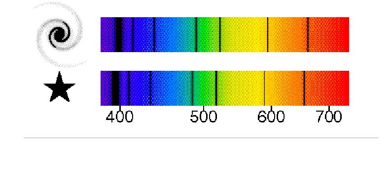
13 Red-shift distnce wvelength

14 Hubble Expnsion: V H R Distnce R Velocity V Accelertion

15 Hubble Expnsion velocity V H R distnce Hubble constnt

16 V H R A specil center?

17 V H R A specil center? Other Origin

18 Prediction fro hoogeneity: The Hubble Lw tie VHR t x x t x x distnce r( x, t) ( t) x & r& x & r H &

19 distnce glxy glxy The Big Bng here now t.7 Gyr tie

20 היכן היה המפץ הגדול? בנקודה אחת? בהרבה נקודות??? היכן המפץ

21 היכן היה המפץ הגדול? בנקודה אחת? בהרבה נקודות? מפץ באינסוף נקודות כל הנקודות מתלכדות לנקודה אחת

22 The Big Bng odel The Stedy Stte odel The Stedy Stte odel

23 Cosic Microwve Bckground Rdition 965

24 COBE 99 Plnk blck-body spectru ( h ν dν I ν ) dν hν / kt c e Nobel Prize 6 to Soot nd Mther Ienergy flux per unit re, solid ngle, nd frequency intervl

25 Hoogeneity nd Isotropy: Robertson-Wlker Metric

26 Metric Distnce B Metric distnce l ( A, B; t) Hubble expnsion in curved spce: dl dl i vi H ( t) l i H ( t) l i H ( t) l dt dt d ln l dt H ( t) locl Hubble lw l( A, B; t) w( A, B) ( t) H ( t) & l cooving distnce i universl expnsion fctor A tt

27 Metric l l l θ const. x. const x cos cos x x x x x x x x + + θ θ l l l l l l l l l In sll neighborhood (loclly flt) Coordinte syste: x, x (d exple) dx dx g dx g dx g d + + l dx dx g dx g dx g d + + l j i ij dx dx g d l Line eleent: Specifies the geoetry uniquely. Exct for depends on the choice of coordintes Orthogonl coordintes: g ij for i j j i ij x x x g ) ( l r The etric: l l l x x

28 Exple: E Coordintes: crtezin sphericl x r sinθ cosφ y r sinθ sinφ z r cosθ intervl d l dx + dy + dz dr + r ( dθ + sin θ dφ ) g crtezin sphericl r r sin dγ θ ngulr distnce dl r dl dl θ φ dr r dθ r sinθ dφ Exple: D sphere ebedded in E : rconst. d l dθ + sin θ d φ Are: da dl dl θ φ r sinθ dθ dφ A π π θ φ da 4π r

29 The Metric of Hoogeneous nd Isotropic Universe (Robertson-Wlker) d l ( t) dw tconst. In cooving sphericl coordintes u r /, θ, φ Isotropy: dw du + σ ( u) dγ d γ dθ + sin θ dφ Three solutions: σ (u) S k ( u) sin( u ) k u k sinh( u) k sinh( x) ( e x e x ) / dl ( t)[ du + S k ( u) dγ ] Spce-tie intervl ds dt ( t)[ du + S k ( u) dγ ]

30 k flt spce (E ) d l ( t) [ du + u ( dθ + sin θ dφ )] u θ π φ π infinite volue

31 k+ closed spce d l ( t) [ du + sin ( u)( dθ + sin θ dφ )] u π θ π φ π For visuliztion: D sphere ebedded in E 4 : (w, x, y, z) D sphere the ebedding is defined by the trnsfortion: consistent with w + x + y + z w z x y cos u sin sin sin u cosθ u sinθ cosφ u sinθ sinφ d l dw + dx + dy + To visulize plot subspce θ π / ( z ) D sphere in w,x,y,z d l ( du + sin uconst. is sphere of cooving rdius u d l sin u ( dθ + sin θ dφ ) A V π π θ φ π sin u dθ sin u A du 4π sin u π sinθ dφ 4π sin u du π u ( t) u dφ ) dz A grows for < u < π/ nd decreses for π/ < u < π x w φ u y

32 k- n open spce d l ( t) [ du + sinh ( u)( dθ + sin θ dφ )]

33 Hoogeneity nd Isotropy Robertson-Wlker Metric ds dt ( t)[ du + S k ( u) dγ ] expnsion fctor cooving rdius r ( t) u ngulr re d γ dθ + sin θ dϕ S k ( u) sin u k + sinh u k u k

34 Rdil ry dγ ds ds dt Redshift dt ν ( t)[ du locl Hubble locl flt λ + S k ( u) dγ ] ± ( t) du u± ( + z ) T t t e o dt ( t) nerby observers long light pth, seprted by δr: δν & δ δv HδrHδuHδt δt ν z λ λ v c For Blck-Body rdition, Plnck s spectru: dn 8πν c Vdν exp( hν / kt) Also for free ssive prticles: p de Broglie wvelength (prticles or photons): like photons: λ h / p p hν / c useful: conforl tie dη dt u η η o e ds ( η)[ dη du S k ( u) dγ ]

35 Horizon u t o dt < lite ( t) t e u( t, t ) u ( t o e horizon o ) liit exists r H ( t) u ( t)) H u H VH 4π Sk ( u) du Exple: EdS (k, Λ) t / u H t dt t / t / r H t M H u H t / Cuslity proble: M H ( trec ) / 4 ( ) ~ M ( t ) H Our Horizon is not cuslly connected: wht is the origin of the isotropy?

36 Friedn s Eqution nd its solutions

37 Newtonin Grvity shell E GM r 4π G v H ρ r r v Hr M 4π ρr M types of solutions, depending on the sign of E H t xiu expnsion, possible only if E< ρ crit H 8 π G ρ ρ crit & 8π G E u r u ρ( t) ε ε ±, independent of r becuse lhs is

38 The Friedn Eqution Newton s grvity: spce fixed, externl force deterining otions Einstein s equtions G 8 µν+λ gµν π GTµν G c left side of E s eq. is the ost generl function of g nd its st nd nd tie derivtives tht reduces to Newton s eqution φ 4π Gρ Grvity is n intrinsic property of spce-tie. geoetry <-> energy density. Prticles ove on geodesics (locl stright lines) deterined by the locl curvture. For the isotropic RW etric ds dt ( t)[ du + S ( u) dγ ] Einstein s tensor Stress-energy tensor & 8πρ k + Λ ss conservtion ρ V const. ρ & Gtt Ttt ρ Tuu T T P k k + G G G uu ϑϑ ϕϕ ϑϑ ϕϕ energy conservtion A differentil eqution for (t) k && & && & k 8πP+Λ conservtion of nuber of photons ρrv ρr N const. ρ r hν Add λ 4 eq. of otion

39 Solutions of Friedn eq. (tter er) *, ny k : & t * Λ & k & * k & t / / * k & + t ( ) k + dη dt & conforl tie + / ( t) * t * * turnround [ cos( η)] [ ηsin( η)] rdition er & (t) t / Λ * & k Λ + * 4π Gρ const. > ccelertion < expnsion forever criticl density ρ H / 8π G H k ρ + 8π G 8π G > collpse Λc Λ > H ( ) & e Ht big bng here & now t

40 Light trvel in closed universe A photon is eitted t the origin (u e ) right fter the big-bng (t e ) dt conforl tie dη photon: ds dη du (t) big crunch π η π/ π t π/ big bng π/ π north pole u south pole

41 H nd t Λ / collpse / / < > << Ht Ht t Ht t k / / ) /( sinh Ht Generl: ) ( sinh ), ( sin...7 ) /( / / > + Λ S S Ht Crrol, Press, Turner 99, Ann Rev A&A, 499

42 Solutions with Cosologicl Constnt Λ & k + + * k Λ> [cosh( Λ t) ] Λ< Λ * [ cosh( Λ * Λ t)] ( tter) && s / t * / Λ Λ> e & 6 Λ / t * / Λ Λ< Λ / t t π / Λ t k- Λ> se syptotic behvior s k Λ< & & & ( t c rd -order polynoil one rel root exists Λ c ) if Λc * / t Λ> e s Λ / t c Λ t c Λ c Λ< t

43 Solutions with Cosologicl Constnt (cont.) Λ & k + + * ( tter) e Λ / t 9 k+ (closed) criticl vlue: Λ c * Letre Λ>>Λ c s Λ>Λ c & > solution for every the rhs t s to be > ΛΛc+ε t ΛΛ c & double root t * & & c c c e Λ / t Einstein s sttic universe (unstble) sttic expnding to infltion Eddington-Letre big-bng expnding to sttic c / t t sttic

44 Solutions with Cosologicl Constnt (cont.) Λ & k + + * ( tter) 9 k+ (closed) criticl vlue: Λ c * <Λ<Λ c & > & < for sll nd lrge for << no solution t cos. const. wins ss ttrction wins Λ & only ttrction t

45 Friedn Eqution k tot + Λ closed/open 8 c kc G H Λ + ρ π & kinetic potentil curvture vcuu 4 r r ρ ρ ρ ρ ρ ρ r ρ + Λ + + k 8 / H c H kc G H k Λ Λ π ρ two free preters, Λ Crrol, Press, Turner 99, Ann Rev A&A, 499 Λ q & && decelerte/ccelerte c g h h G H π ρ Flt: k tot Λ ) ( + ) ( / H H + Λ

46 Drk Mtter nd Drk Energy vcuu repulsion? Λ unbound bound ss - ttrction

47 Cosologicl Constnt: Newtonin Anlog vcuu energy density Λ 4πρ Λ M Λ 4π ρ r Λ Λr force per ss on shell F M r rˆ Λ Λ r rˆ vs. M r ˆ r potentil r φ Fdr Λ r 6 vs. M r in Einstein s eqs. & 8π ρ k + Λ && 4π ρ + Λ

48 if ρ Accelertion, pressure, energy density FRW: dointes if ρ dointes r 8 π & ρ ( k Energy chnge by work d( ρ c ) pd( ) () if ρ ) 4π p && ρ+ c 4 ρ ρλ + ρ + ρr G () 4π ρ ρ p & 4 4 () 8π ρr ρ ρ & r pr rc () 8π ρλ const. pλ ρλc && ρλ Λ dointes + Construct sttic odel: de Sitter: p/c Quintessence Λ ω ωρ ρ p ρ p 8π & in FRW : ρ kc () p && ρ ρ > Λ ρ ρλ ρ c H & / Λc / for infltion need &> & to exceed r ct & r ω</ h Ht e h dv k +

49 Future SN Cosology Project

50 Drk Energy w ccelertion WMAP_ Λ WMAP_

51 Friedn Eqution Hoogeneity + Grvity ( G Λ g 8 ) H & kc c + 8π Gρ µν µν π GTµν Λ kinetic potentil curvture vcuu ρ ρ + ρ r ρ 4 ρ ρr ρr ρ crit + k + Λ ρ kc Λc c k Λ H / 8 G H H π ~ 9 g c two free preters +Λ closed/open q tot && & Λ k decelerte/ccelerte

52 Solutions of Friedn eq. & * k : t sll : k / t / * 4π Gρ const. ny k lrge, k : t << k t + * * H d η dt / ( t ) [ cos( η)] [ ηsin( η)] & Ht e Λc tter er, Λ (t) conforl tie ccelertion Λ big bng here & now t & 8π Gρ kc Λc H + > +k < > collpse + Λ expnsion forever

53 Accelertion by cosologicl constnt: & 8π Gρ kc Λc H + q +Λ k && & Λ distnce > Λ e Ht Λ < > Big Bng here & now tie

54 Generlized Drk Energy Energy conservtion during expnsion: Cosologicl constnt: d( ρtotc ) p d( ρtot ρ Λ const. ) Eqution of stte: pρ c negtive pressure Generl eq. of stte: Λ p wρ c w e.g. Quintessence w( x, t)? &> & w< / & FRW ( k ) 8πG ρ tot 4π G p && ρ+ c