Investigating Non-Periodic Solids Using First Principles Calculations and Machine Learning Algorithms

Transcript

1 Investigating Non-Periodic Solids Using First Principles Calculations and Machine Learning Algorithms The Harvard community has made this article openly available. Please share how this access benefits you. Your story matters. Citation Accessed Citable Link Terms of Use Çubuk, Ekin Dou Investigating Non-Periodic Solids Using First Principles Calculations and Machine Learning Algorithms. Doctoral dissertation, Harvard University, Graduate School of Arts & Sciences. October 17, :39:11 AM EDT This article was downloaded from Harvard University's DASH repository, and is made available under the terms and conditions applicable to Other Posted Material, as set forth at (Article begins on next page)

2

3

4

5

6

7

8 x Y x

9 χ D =0 χ D χ T χ O

10 D 2 d =2 D 2 σ AA C

11 D 2 D 2 d AA T T =0.1, 0.2, d =2 d =3 T =0.4, D 2 D 2 D 2 D 2 T =0.4 D 2 T g AB g BA

12 G A B (i; rab ) r AB rab g AB g BA Ψ B AB (i;2.07σ AA, 1, 2) i T = 0.47 ρ = 1.20 p p T =0.47 p p T =

13 p c T = 0.47 ρ = 1.20 p =0.2 p c p c = T = 0.47 ρ =1.20 S > 0

14 P R (S) T = P R (S) dq(s, t)/dt T =0.47 T =0.58 P R (S) 1/T S 3 S 3 P R /P 0 E/T E Σ P R (S) =exp(σ E/T ) S T 0 T m 0 ρ =1.15, 1.20, 1.25, 1.30 T 0 = T m 0 T = P R (S)

15 S 0 3 t =0 t = 1000τ S 0 3 S 0 3 r

16 q(s, t) T =0.47 T = T =0.45 T =0.70 γ E(S) S T = 0.47 ρ =1.20 f rrev T =0.47 T =

17 N T N O ξ =1.2 ξ =1.1 i r i S i r S P (cos θ) r S g AA (r) g AB (r)

18

19

20

21

22

23 1

24 3 N at N at

25

26

27 H = i i,i I 2 2 2m i + 1 e 2 e 2 i j i j Z I e 2 I i 2 2 2M I + 1 Z I Z J e 2 I 2 I J I J M I Z I I I m e i i e HΨ( I, i )=EΨ( I, i ), Ψ( I, i ) ( )

28 10 23 Ψ( I, i ) m e

29 H = i i 2 2 2m i + 1 e 2 e 2 i j i j i,i 2 2 2m i + 1 e 2 e 2 i j i i j Z I e 2 I i V ion ( i ) Ψ( i )=Ψ( 1, 2,... N ) 3 N

30 Ψ( i ) n ( ) n ( ) =N Ψ ( 1, 2,... N )Ψ( 1, 2,... N )d 2 d 3...d N V( ) n ( ) V 1 ( ) V 2 ( ) n ( ) H 1 H 2 Ψ 1 Ψ 2 V 1 ( ) V 2 ( ) E 1 E 2 E 1 = Ψ 1 H 1 Ψ 1 E 2 = Ψ 2 H 2 Ψ 2 E 1 < Ψ 2 H 1 Ψ 2 = Ψ 2 H 2 V 2 +V 1 Ψ 2 = Ψ 2 H 2 Ψ 2 + Ψ 2 V 1 V 2 Ψ 2 = E 2 + Ψ 2 V 1 V 2 Ψ 2

31 E 2 < Ψ 1 H 2 Ψ 1 = Ψ 1 H 1 V 1 +V 2 Ψ 1 = Ψ 1 H 1 Ψ 1 + Ψ 1 V 2 V 1 Ψ 1 = E 1 + Ψ 1 V 2 V 1 Ψ 1 E 1 + E 2 <E 1 + E 2 + Ψ 1 V 2 V 1 Ψ 1 + Ψ 2 V 1 V 2 Ψ 2 n ( ) Ψ 1 V 2 V 1 Ψ 1 = Ψ 2 V 2 V 1 Ψ 2 = n ( )[V 2 ( ) V 1 ( )] d E 1 + E 2 <E 1 + E 2 n ( ) R 3 n ( )

32 H = F [n( )] + V( )n( )d F [n( )] F [n( )] n( ) V( ) F [n( )] n ( ) Ψ( i ) Ψ( i ) n( ) = i φ i ( ) 2 φ i ( ) F [n( )] F [n( )] = T s [n( )] + E H [n( )] + E xc [n( )], T s [n( )] E H [n( )] E xc [n( )]

33 E xc [n( )] F [n( )] T s [n( )] T s [n( )] E xc [n( )] ] [ 2 2 +V eff (,n( )) φ i = ϵ i φ i ( ), 2m e V eff (,n( )) = V( )+e 2 n( ) d + δe xc[n( )], δn( ) φ i ( ) n( ) V eff

34 E xc [n( )] R 3Nat F [n( )]

35

36

37 2

38 x x 2

39 1 x 2.5 x 2.5 x x 2.5 x =3.75 x x x

40 x x = x x x =4.25 x x x 2 ζ

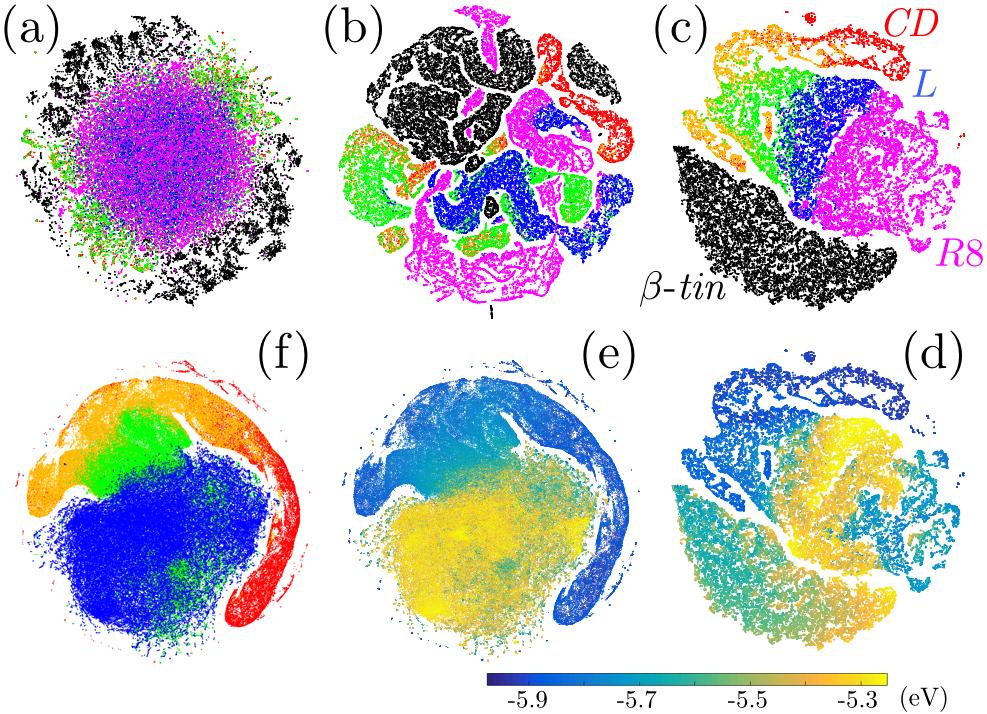
41 (a) (b) Volume expansion pure a Si Formation energy (ev/si atom) Li concentration x Li concentration x 3 4 6B;m`2 kxr, U V _2T`2b2Mi ibp2 mmbi +2HHb Q7 i?2 bi`m+im`2b M Hvx2/ Uv2HHQr bt?2`2b `2 ab iqkb M/ Tm`TH2 bt?2`2b GB iqkbvx U#V p2` ;2 7Q`K ibqm 2M2`;v b 7mM+iBQM Q7 GB +QM+2Mi` ibqmx 6BHH2/ +B`+H2b +Q``2bTQM/ iq i?2 +QM+2Mi` ibqmb i r?b+? i?2 bi`m+im`2b `2 b?qrm BM U VX h?2 BMb2i BM U#V b?qrb i?2 pqhmk2 `2H ibp2 iq i?2 BMBiB H pqhmk2 h?2 `2bmHib `2 p2` ;2 p Hm2b Qp2` Ry bi`m+im`2b i 2 +? p Hm2 Q7 xx h?2 bi M/ `/ /2pB ibqm 7Q` 2 +? TQBMi Bb bk HH2` i? M i?2 K `F2` bbx2x i?2b2 TQbBiBQMb- r2 B/2MiB7v ab iqkb rbi? i?2?b;?2bi MmK#2` Q7 ab M2B;?#Q`b i 2 +? GB +QM+2Mi` ibqmx q2 i?2m TB+F QM2 Q7 i?2b2 ab iqkb M/ QM2 Q7 Bib ab M2B;?#Q`b ` M@ /QKHv M/ BMb2`i i?2 GB iqk HQM; i?2 2ti2MbBQM Q7 i?2 +?Qb2M ab@ab #QM/ i /Bb@ i M+2 TT`QtBK i2hv 2[m H iq i?2 #QM/- M/ `2H t i?2 bi`m+im`2 b /2b+`B#2/X i 2 +? x p Hm2- r2 +QMbi`m+i2/ Ry /Bz2`2Mi bi`m+im`2b # b2/ QM bi`m+im`2b i i?2 T`2pBQmb x p Hm2- rbi? i?2 TQbBiBQM Q7 2 +? GB iqk +?Qb2M ` M/QKHv KQM; i?2 p BH #H2 TQbB@ ibqmb /2}M2/ #Qp2X h?2`2 `2 K Mv bm+? TQbBiBQMb BM i?2 M2irQ`F- r?b+? ;Bp2b #`Q / ` M;2 Q7 BMBiB H bi`m+im`2b 7Q` i?2 }`bi HBi?B ibqm bi2tx q2 b?qr }p2 Q7 i?2 bi`m+im`2b 7`QK Qm` + H+mH ibqmb BM 6B;X kxru VX h?2 KQmMi Q7 GB r b BM+`2 b2/ BM bi2tb Q7 x = 0.125X q2 ``Bp2/ i i?2 p Hm2 Q7 x 7i2` 2tT2`BK2MiBM; iq /2i2`@ KBM2 i? i i?bb +?QB+2 /Q2b MQi z2+i i?2 `2bmHiBM; bi`m+im`2x 6Q` bk HH p Hm2b Q7 x- RN

42 E f (x) x E f (x) =(E Lix Si E Li N Li E Si N Si )/N Si E Lix Si E Li E Si N Li N Si N Si = 64 E f (x) x x x =3.75 x 15 4 V E f (x 1 ),E f (x 2 ) x 1,x 2 V = 1 e E f (x 2 ) E f (x 1 ) x 2 x 1 e

43 E f (0) E f (3.75) V E f (3.75) E f (2) V E f V Number of neighbors (a) Li tot Si Si Si tot Li Si Si Li Li Li Rings per atom (b) 6 Si(x4) Li Li concentration x Li concentration x Y x

44 x x =4.25 x =2 x 2 x =2.2 x =2.2 x

45 x x =0 x 0.5 x 2 x x x 4.25 x 2

46 χ D χ D χ D =0 Shape measures (a) Li concentration x D O T Tetrahedricity n=1 n=2 (b) Li concentration x Fraction of Si χ D =0 x = 0 χ D χ D x x

47 x χ D χ D χ T χ O χ D χ T χ O χ I = 1 ( ei N p e 2 e ) 2 j λ i λ j i<j I = e i,j e N p λ i,j = 1 λ i,j = 2 i j χ D x χ O χ T χ D χ T χ O x 2 2 x 4.25 χ T χ O x

48 χ T χ O x x x x = O D T χ D χ T χ O 15 4 χ T χ T =0.020 χ T χ T =0.020 χ T χ T

49 x 2.25 x = 3.75 χ T χ T x 3.25 x = χ T χ T < x =

50 x 2 x = x 2 x 2 2 x 4.25

51 3

52

53 Atomic&coordinates Symmetry&functions Input& layer Hidden& layer Output& layer E 1 E T E 2

54 β

55 (23, ) 1.5 E i N n N n E i

56 N n N n N n = 60 N n =

57 β

58 β 11.7 β β β β

59 3 N a N a 3 43) = n th n th

60 β

61 β

62 β β β

63

64 4

65

66 i G X Y (i; µ) = j e (R ij µ) 2 /L 2 Ψ X YZ(i; ξ,λ,ζ) = j e (R2 ij +R2 ik +R2 jk )/ξ2 (1 + λ cos θ ijk ) ζ k R ij i j θ ijk i j k L µ ξ λ ζ X Y Z i X j Y k Z

67 µ ξ λ ζ G Ψ R S c R S c µ, ξ, ζ, λ G X A GX B µ ΨX AA ΨX AB, Ψ X BB (ξ,λ,ζ) µ 0.3σ AA 5.0σ AA 0.1σ AA ξ,ζ, λ G X Y (i; µ) ΨX YZ (i; ξ,λ,ζ) N M G X Y ΨX YZ µ ξ λ ζ M = 160 {F 1,, F N } F i i t i R M n

68 Structure"function"parameters"for"Ψ YZ ξ"(σ AA ) ζ λ t i t i + t R M

69 C C C C>0.1 i D 2 (i) min Λ 1 (R ij (t + t) ΛR ij (t)) 2 z, j t j R D c i R ij i j z R D c Λ D 2 RD c t R D c t D 2 D2 D % D,0 2 D 2 D 2 D 2 T = 0.4 d = 2 D 2 D2 = 0.3σ2 AA D 2 = 0.28σ2 AA D 2

70 rdered cles to is dehe two e consented titutes icle i, dom a nd catrrange etween d time d. ng set, cheme se the h conft pars been rticles ssified em on no exdapted ct; the where ations. nsensim was 2 6B;m`2 9XR, U+QHQ` QMHBM2V am Tb?Qi +QM};m` ibqmb Q7 i?2 irq bvbi2kb bim/b2/x S `ib+h2b `2 +QH@ 2 Q`2/ ;` v `2/ ++Q`/BM;online) iq i?2b` DKBM p Hm2X S `ib+h2b B/2MiB}2/ b bq7i #v i?2 aojof `2 the QmiHBM2/two FIG. 1. iq (color Snapshot configurations BM #H +FX U V bm Tb?Qi Q7 i?2 TBHH ` bvbi2kx *QKT`2bbBQM Q++m`b BM i?2 /B`2+iBQM BM/B+ i2/x U#V systems Particles are colored bm Tb?Qi Q7studied. i?2 d = 2 b?2 `2/i?2`K H G2MM `/@CQM2b bvbi2kx gray to red according 2 to their Dmin value. Particles identified as soft by the SVM 2 2 p Hm2 Q7 = 0.28σ(a) iq MQM@ {M2 /BbTH +2K2Mi Q`@ arei?`2b?qh/ outlined indkbm-y black. A snapshot of the pillar Q7system. AA +Q``2bTQM/b 2 2 Compression occurs in the direction indicated. (b) A snapshot /2` DKBM-y = 0.53σ AA X h?2 DKBM-y 7Q` Qi?2` i2kt2` im`2b r2`2 b+ H2/ HBM2 `Hv rbi? of i2kt2` im`2the d = 2iQ sheared, thermal Lennard-Jones system. ;Bp2 D2 (T ) 0.7T σ 2 X KBM-y AA. / h?2 i` BMBM; b2i Bb ;Bp2M #v {(F1, y1 ),..., (FN, yn )}- r?2`2 Fi 4 Fi1,..., FiM `2 i?2 p Hm2b Q7 i?2 bi`m+im`2 7mM+iBQMb i? i /2b+`B#2 i?2 HQ+ H M2B;?#Q`?QQ/ Q7 T `ib+h2 ix plate fixed and ithe toprbi?bm plate is M/ driven the yi = 1is B7 i?2 M2B;?#Q`?QQ/ `2 `` M;2b ibk2 tyi = 1 into Qi?2`rBb2X q2 pillar BKatiQ a}m/constant speed v0 b2t ` i2b = mm/s. The yipillars?vt2`th M2 w F b =of 0 i? i i?2 TQBMib rbi? /Bz2`2Mi X ReN X.m2 iq i?2 are h?2 composed ofr ba BKTH2K2Mi2/ bidisperse mixture of approximately aoj H;Q`Bi?K mbbm; i?2 GA"aoJ T +F ; rigid grains with size ratio and`2 `` M;2 the large partibiq+? bib+ M im`2 Q7 `2 `` M;2K2Mib UBX2X MQi HH bq7i3:4 T `ib+h2b i 2p2`v ibk2 cles having a radius daa = particles BMi2`p HV i?2`2 /Q2b MQi 2tBbi of?vt2`th M2 i? i0.3175cm. T2`72+iHv b2t ` i2bthese i?2 irq /Bz2`2Mi have elastic interactions with +H bb2bx 6Q` i?bb and `2 bqm-frictional T2M Hiv T ` K2i2` C Bb BMi`Q/m+2/ M/ r2each }M/ i?2other, QTiBK H as well as frictional interactions with the substrate, making the identification of flow defects using vibrational modes 93 impossible. A camera is mounted above and captures images at 7 Hz throughout the compression. We construct our training set from compression experiments performed on ten di erent pillars. We select

71 0.75 Avg. accuracy D 2 min,0 D 2 σ AA 1 2 wt w + C N ξ i, i=1 y i (w T φ(f i )+b ) 1 ξ i ξ i 0 φ(f i ) K(F i, F j )=φ(f i ) φ(f j ) K(F i, F j )= F i F j K(F i, F j )= { γ F i F j 2} γ C

72 C C > 0.1 C =1 C hard particles Fraction soft particles C value used in this study C C d =3

73 Accuracy training set test set Size of training set 10 4 d = 2 v 0 =0.085 d AA =0.3175

74 D 2 R D c =1.5 d AA D 2 =0.25d2 AA y y + δy v 0.04 d =2 d =3 σ AA =1.0 σ AB =0.88 σ BB =0.8 ϵ AA =1.0 ϵ AB =1.5 ϵ BB = σ AA σ AA ϵ AA τ = mσaa 2 /ϵ AA τ ρ =1.2 τ ϵ AA /k B k B d = 2 T =0.1, 0.2, 0.3, 0.4 γ = 10 4 /τ d =3 T =0.4, 0.5, 0.6 T G =0.33 d =2 T G =0.58 d =3

75 (a) (b) (c) (d) 0.6 P D 2 min/(d 2 AA) D 2 min/(t 2 AA) D 2 min/(t 2 AA) D 2 min/(t 2 AA) D 2 D 2 d AA T T = 0.1, 0.2, d =2 d =3 T =0.4, d =2 t =2τ D 2 R D c = 2.5σ AA t =2τ d =3 D 2 d = 2 d = P (D 2 ) D2 d =3

76 P (D 2 ) D2 d =2 d =3 P (D 2 ) T D 2 Tσ2 AA D 2 v2 T d =2 T =0 T =0.1 T =0.4

77 14% 76% 62% 1.0 D min,0 0.8 P Dmin 2 /(T AA 2 ) D 2 D 2

78 T =0.4 P D 2 d = 2 T = 0.1 G X Y (i; µ) g XY (r) = lim L 0 G X Y (i; r) /2πr g(r) g(r) L =0.1σ AA

79 P D /(σ 2 AA 2 ) D /(Tσ 2 AA 2 ) D 2 D 2 T = 0.4 D 2 T g(r) G X Y (i; µ) G B A (i; rab ) r AB g BA(r) G B A (i; rab )/r < 1/2 H 0 G B A (i; rab )/r > 1/2 H 1 H 1 H 0 Ψ B AB (i;2.07σ AA, 1, 2)

80 1.0 B AB (i; 2.07 AA, 1, 2) P for soft hard particles (blue), and H1 gaa (r) gba (r) shown in Fig. 3(c). Physically is large when there are many 0.5 the central particle that lie wi small angles between them, suc A and one is of species B. The a single category (one peak, r 0.0 H1 -type hard particles defined above have very di erent distri gab (r) gbb (r) peaks). Unlike before, here th H0 hard particles have very di e 0.25 soft particles and H1 hard part butions. Bond-angle information between soft particles and H0 not between soft particles and 0.0 To fully distinguish between s both radial and bond-angle info r/ AA r/ AA particles have environments th fewer particles in their nearest n FIG. 3. (color online) Radial distribution functions averaged 6B;m`2 9X3, U+QHQ` QMHBM2V _ /B H /Bbi`B#miBQM 7mM+iBQMb p2` ;2/ Qp2`? `/ U#H +F HBM2bV Q` bq7ibetween adjacent particle angles over hard (black lines) or soft (red lines) particles. gab and U`2/ HBM2bV T `ib+h2bx ggba M/ gba Q7 bq7i T `ib+h2b `2 MQito2[m H 2 +?since Qi?2`they bbm+2 i?2v In `272` iq AB of soft particles are not equal each iq other summary, we have presented /Bz2`2Mi FBM/b Q7 `2;BQMb, M2B;?#Q`b bq7i T `ib+h2b 7`QK bt2+b2b of M/ T `ib+h2b refer to di erentq7kinds of regions: neighbors softm2b;?#q`b particles Q7 bq7i identifying flow defects in disorde 7`QK bt2+b2b "- `2bT2+iBp2HvX from species A and neighbors of soft particles from species B, we have focused on the short-ti respectively. ture with particle rearrangement 1.0 M/ H1? `/ T `ib+h2b U;`22MV- b?qrm BM 6B;X ju+vx should H0? `/ T `ib+h2b U#Hm2VS?vb@ shed light on the connect tural evolution and the correlati BA, 1, 2) Bb H `;2 r?2m i?2`2 `2 K Mv T B`b Q7 M2B;?#Q`b time and space [31] over longer t B+ HHv- ΨB Q7 i? AB (i; 2.07rT2 F ing liquids. We also note that +2Mi` H T `ib+h2 i? i 0.5 HB2 rbi?bm /Bbi M+2 ξ rbi? bk HH M;H2b #2ir22M i?2k- specific bm+? i? i particles that will partic at a later time; rather, we ident QM2 Bb Q7 bt2+b2b M/ QM2 Bb Q7 bt2+b2b "X h?2 bq7i T `ib+h2b 7 HH BMiQ bbm;h2ticles + i2@that are likely to rearran 0.25 more useful in thermal and/o ;Q`v UQM2 T2 F- `2/V r?bh2 M/ `/ T `ib+h2bĝ/2}m2/ 7`QKis` /B H fluctuations lead to stochasticity /Bz2`2Mi 8 12 /Bbi`B#miBQMb U#Hm2 0.4 M/ Our method relies on local s BM7Q`K ibqm #Qp2Ĝ? p2 p2`v ;`22M1 T2 FbVX lmhbf2 be applied directly to snapsho B B GA (i; rpeak ) BA (i; 2.07 AA, 1, 2) #27Q`2-?2`2 i?2 bq7i T `ib+h2b M/ i?2 H0? `/ T `ib+h2b? p2 p2`v /Bz2`2Mi /Bbi`B#m@ tems, in contrast to previous m AB FIG. 4. (color online) (a) Distribution of GA B (i; rpeak ), proporproach also scales linearly with AB ibqmb r?bh2 bq7i T `ib+h2b H1? `/weighted T `ib+h2bdensity? p2 bbkbh ` tional to M/ the gaussian at rpeak, /Bbi`B#miBQMbX for soft (red) "QM/@ M;H2 N, while vibrational mode appr AB and hard (blue/green) particles. rpeak corresponds to the first efficient identification of flow de BM7Q`K ibqm i?2`27q`2 bq7i T `ib+h2b M/ `/ T `ib+h2b peak /BbiBM;mBb?2b of gab or gba. #2ir22M (b) Distribution of B AB (i; 2.07 AA, 1, 2), ing phenomenological approache proportional to the density of neighbors with small bond anflow#2@ defects [6, 32 34]. Previous #mi MQi #2ir22M bq7i T `ib+h2b M/ `/ T `ib+h2bx hq 7mHHv /BbiBM;mBb? gles near a particle i,1 for soft (red) and hard (blue/green) learning methods in physics hav particles. The inset shows examples of configurations with tion [25, 35, 36] or on optimizati corresponding radial and bond orientation properties, where dark (light) gray neighbors 83 are of species A (B). 40]. Our approach shows that su detecting subtle correlations can gain conceptual understanding n features a single peak, that for hard particles is bimodal. tional approaches. This indicates the existence of (at least) two distinct E.D.C. and S.S.S. contributed populations of hard particles which we divide into two thank Amos Waterland, Carl Go AB groups: one with GB and Franz Spaepen for helpful dis A (i; rpeak )/r < 1/2 (blue) that we will B AB

81 not between soft particles and H To fully distinguish between sof both radial and bond-angle inform r/ AA r/ AA particles have environments tha fewer particles in their nearest ne FIG. 3. (color online) Radial distribution functions averaged angles between adjacent particles. over hard (black lines) or soft (red lines) particles. gab and gba of soft particles are not equal to each other since they In summary, we have presented refer to di erent kinds of regions: neighbors of soft particles identifying flow defects in disorder from species A and neighbors of soft particles from species B, we have focused on the short-tim respectively. ture with particle rearrangements. should shed light on the connectio 1.0 tural evolution and the correlatio time and space [31] over longer ti 0.75 ing liquids. We also note that specific particles that will particip 0.5 at a later time; rather, we identif ticles that are likely to rearrange 0.25 is more useful in thermal and/or fluctuations lead to stochasticity i Our method relies on local str be applied directly to snapshots B GB A (i; rpeak ) BA (i; 2.07 AA, 1, 2) tems, in contrast to previous m AB FIG. 4. (color online) (a) Distribution of GA B (i; rpeak ), proporab proach also scales linearly with th 6B;m`2 9XN, U+QHQ` QMHBM2V U V.Bbi`B#miBQM Q7 GA (i; r )T`QTQ`iBQM H iq i?2 ; mbbb M r2b;?i2/ AB B T2 F tional to the gaussian weighted density at rpeak, for soft (red) AB AB N, while /2MbBiv i rt2 F - 7Q` bq7i U`2/V M/? `/ U#Hm2f;`22MV T `ib+h2bx rt2 F +Q``2bTQM/b iq i?2 }`bi T2 Fvibrational mode approa AB and hard (blue/green) particles. rpeak corresponds to the first B efficient identification of flow def Q7 gab Q` gba X U#V.Bbi`B#miBQM 2.07σ T`QTQ`iBQM H iq i?2 /2MbBiv Q7 M2B;?#Q`b B AA, 1, 2)-of AB.(i; peak of gab Q7 or Ψ gba (b) Distribution AB (i; 2.07 AA, 1, 2), ing phenomenological approaches rbi? bk HH #QM/ M;H2b M2 ` T `ib+h2 i- density 7Q` bq7i of U`2/V M/? `/ U#Hm2f;`22MV h?2 BMb2i proportional to the neighbors with small bondt `ib+h2bx anflow defects [6, 32 34]. Previous a b?qrb 2t KTH2b Q7 +QM};m` ibqmb rbi? +Q``2bTQM/BM; ` /B H and M/ hard #QM/ (blue/green) Q`B2Mi ibqm T`QT2`iB2b- r?2`2 gles near a particle i, for soft (red) learning methods in physics have / `F UHB;?iV ;` v M2B;?#Q`b `2 Q7 bt2+b2b U"VX examples of configurations with particles. The inset shows tion [25, 35, 36] or on optimizatio corresponding radial and bond orientation properties, where dark (light) gray neighbors are of species A (B). 40]. Our approach shows that such ir22m bq7i M/? `/ T `ib+h2b- #Qi? ` /B H M/ #QM/@ M;H2 BM7Q`K ibqm Bb M22/2/X aq7isubtle correlations can a detecting gain conceptual understanding not T `ib+h2b? p2 2MpB`QMK2Mib i? iĝ i KBMBKmKĜ? p2 72r2` T `ib+h2b BM i?2b` M2 `2bi features a single peak, that for hard particles is bimodal. tional approaches. This indicates the existence of (at least) two distinct E.D.C. and S.S.S. contributed eq M2B;?#Q` b?2hh M/populations H `;2` M;H2b /D +2Mi T `ib+h2bx of #2ir22M hard particles which we divide into two thank Amos Waterland, Carl Goo B AB groups: one with GA (i; rpeak )/r < 1/2 (blue) that we will and Franz Spaepen for helpful disc AB call H0 -type, and one with GB supported by the UPENN MRSE A (i; rpeak )/r > 1/2 (green) 9Xe *QM+HmbBQM that we will call H1 -type. Radial information therefore (S.S.S., J.M.R.), NSF DMR-1305 distinguishes between soft particles and H1 hard particles partment of Energy, Office of B but not between soft and H hard particles. Division of Materials Sciences a 0 AM bmkk `v- r2? p2 T`2b2Mi2/ MQp2H JG K2i?Q/ 7Q` B/2MiB7vBM; ~Qr /272+ib BM /Bb@ We now consider the distribution of Award DE-FG02-05ER46199 (A.J Q`/2`2/ bqhb/bx q2 MQi2 i? i r2? p2 7Q+mb2/ QM i?2 b?q`i@ibk2 +Q``2H ibqm Q7 bi`m+@ P 0.0 im`2 rbi? T `ib+h2 `2 `` M;2K2MibX >Qr2p2`- Qm` K2i?Q/ b?qmh/ b?2/ HB;?i QM i?2 +QM@ M2+iBQM #2ir22M HQ+ H bi`m+im` H 2pQHmiBQM M/ i?2 +Q``2H ibqm Q7 `2 `` M;2K2Mib BM ibk2 M/ bt +2 R Qp2` HQM;2` ibk2 b+ H2b BM ;H bb7q`kbm; HB[mB/bX q2 HbQ MQi2 i? i r2 + MMQi T`2/B+i i?2 bt2+b}+ T `ib+h2b i? i rbhh T `ib+bt i2 BM `2 `` M;2K2Mib i H i2` ibk2c ` i?2`- r2 B/2MiB7v TQTmH ibqm Q7 T `ib+h2b i? i `2 HBF2Hv iq `2 `` M;2X h?2 H i@ i2` [m MiBiv Bb KQ`2 mb27mh BM i?2`k H M/fQ` b?2 `2/ bvbi2kb- bbm+2 ~m+im ibqmb H2 / iq biq+? bib+biv BM `2 `` M;2K2MibX 8N

82 N N 3

83 5 T 0

84 T 0 M = 166 M R M i M τ α

85 S i i R M S i > 0 i S i < 0 d =3 ρ T A 6, 000 T R M S i (t) i t 30, 000τ ρ T σ AA =1.0 σ AB =0.8 σ BB =0.88 ϵ AA =1.0 ϵ AB =1.5 ϵ BB =0.5 m A = m B =1 τ = m A σaa 2 /ϵ AA k B =1 2.5σ AA τ τ

86 ρ ρ p p t R = 10τ A = [t t R /2,t] B =[t, t + t R /2] p (t) = ( r i r i B ) 2 A ( r i r i A ) 2 B A B A B p p 0.05

87 p t 1 p t 2 r = r t (t 2 ) r i (t 1 ) t = t 2 t 1 phop ri(t) ri(0) (a) (b) t/ T =0.47 ρ =1.20 p p t r p T =0.47 p p r t p P R (S) dq/dt p

88 PH»Dr»L »Dr» PHDtL Dt p T =0.47 p a P R (S) a r t r p r p p t p p p 0.2 τ R (T ) τ R (T ) T τ R (T )

89 X»Dr»\ * p hop XDt\ * p hop p T = p >p c =0.2 p c S > 0 T =0.47 p c p c % p 0.2 p c 0.2 p c

90 P (S >0) p c p c T =0.47 ρ =1.20 p =0.2

91 DE Ì Á Ûı Û ı ÙÌ Á ÁÁ ÛÌ ı Û Ûıı ıù Û ÁÚ Ù Ï ÚÚ Ï Ï ÚÚÚ Á Á ÙÙÙ Ì ÌÌ ÌÌ Ì Û ÛÛ Û ı ıı ı ÏÏ Ï Ú ÙÙ Á Ú Ú Ù Ûı ı Ê Ï ÊÊÊ ÏÁ ÚÚÚÚ ÏÏÏÏ Ù Á Û Ù Û Ù Ù ÌÌÌÌÌÌ ÁÁÁÁ Û ı ıı ÛÌÌ Û ıı Û Û ı ÙÙ ÚÚ Ê Ï Ú ÙÙÙ Ì ÁÁÁ Ú ÊÊÊÊ ÚÚÚÚÚÚÚÚ ÁÁ Ù ÊÊ ÊÊÊÊÊÊÊ ÏÏÏÏÏÏÏÏÏÏÏ ÙÙ Á Ûı Ì ÛÛ ıı ÌÌ ı ÛÛ ÁÁÁÁ Ù Ì ı Ì Û ÌÌ Û ı ÙÙÙÙ Á Ûı ÁÁÁ Ú ÏÏÏ ÚÚ ÙÙ ÙÙÙ ÌÌÌÌÌÌÌÌÌÌ ÛÛ ııı ÛÛ ı Û ÛÛ ıı ı Û ÚÚÚ Ù ÁÁÁÁÁÁÁÁÁÁ ÙÙÙÙÙÙÙÙÙ Û ı ı ÛÛÛ ıìì ı ÌÌÌÌÌÌÌÌ ÚÚÚÚÚÚÚÚÚÚ ÛÛÛÛ ıııı ÁÁ ÏÏÏÏÏÏÏÏÏÏÏÏÏ Á ÚÚ Ù Ù ÌÌ ÙÙÙ ÙÙÙÙÙÙÙÙ ÏÏÏÏÏ ÏÏÏÏ ÚÚÚÚÚÚÚÚÚÚÚ ÌÌÌÌÌÌÌÌÌÌÌÌ Û ı Û ıııııııııııııı ÛÛÛÛÛÛÛÛÛÛÛ ÛÛ ÛÛÛÛÛÛ ııı ÚÚ ÙÙÙÙ ÁÁÁÁÁÁÁÁÁÁÁÁÁÁÁÁÁÁÁÁ ÚÚÚÚÚÚÚ ÙÙÙÙÙ ÌÌÌÌ ııı ÏÏÏÏÏÏÏÏÏÏÏÏÏ ÊÊÊ ÊÊÊÊÊÊÊÊÊÊÊÊÊÊÊÊÊÊÊÊÊÊÊÊÊÊÊÊÊÊÊÊÊÊÊÊÊÊÊÊ S loghp0l Ù Á ÛÌ Á Ú Ú ÏÊ Ê Ê Ê ÊÊÊ ÏÏ ÚÚ ÏÏÏ Ú Ù ÙÙ Ì Û Á Ì Ì Ú Û ÙÌ Ù Á Á ÁÌ ÏÚÚ Ï Ê Ú Á Û Ù Ì Û Ù Ù Ì Û Ù ÁÁ Ê ÏÏÏÏ ÏÏ Ú ÏÏ Ï ÊÊÊÊÊÊÊÊÊÊÊÊ Ú Ú Ì Ì Û Ì ÛÛÛ Û Ù Ù ÚÛ ÚÚ ÚÚÚ ÙÙ Ù ÁÁ ÁÁÁÁ Ì Ì ÙÙÙ ÏÏÏÏÏÏÏÏ Ú ÙÙ ÚÚ Ù Ì ÛÛ Ì Ì Û ÛÛ Ì Á Á Á Ì ÁÁ ÌÌ Á ÚÙÙÙÙ Ê Û ÚÚÚÚ ÊÊÊÊÊÊÊ Á ÏÏ ÚÚ ÛÌ ÛÛ ÛÌ Û Ì Ì ÛÌ ÁÁÁÁÁ Ù ÙÙÙ ÏÏÏ ÚÚÚ ÛÌ ÙÙÙ ÊÊ ÁÁÁÁÁÁÁÁÁ ÏÏÏÏÏÏÏÏ Ú ÚÚÚÚÚÚÚÚ Ù ÙÙÙÙÙÙÙ ÛÛÛ ÌÌ ÌÌ Û Ì Ì Ì Û ÛÛ Ì Ì Û ÊÊÊÊÊÊÊÊÊÊ Û Û Ì ÛÌ Ì ÏÏ Ú ÛÛÛÛ Ì Á Ù ÌÌÌ Ï ÁÚ Ù Á Û ÚÙ ÊÊÊ ÁÁÁ ÚÚÚ ÙÙÙ ÚÚÚÚÚ ÙÙÙÙÙÙÙÙ Ì Û Ì Û Ì ÛÛÛÛÛÛÛÛÛÛ ÌÌ ÏÏÏÏÏÏÏÏÏÏÏ ÁÁÁÁÁÁÁÁ ÌÌÌÌÌÌÌÌÌÌ ÚÚÚ ÊÊÊÊÊÊÊÊÊÊ ÏÏ ÁÁ ÚÚÚÚ ÙÙ ÊÊ Û ÏÏÏÏÏÏÏ ÁÁÁÁÁÁÁ ÙÙÙÙÙÙÙ ÊÊÊÊÊÊÊ ÌÌ ÚÚÚÚÚ ÛÛÛ ÌÌÌÌ Û ÛÛ S p c p c = Ê Ê Ê Ê Ê Ê Ê Ê Ê Ê Ê Ê Ê Ê e1 8.0 E1 8 Ê Ê Ê Ê Ê 7.0 Ê log p c p c y i =1

92 τ α y i =0 {(F 1,y 1 ),...,(F N,y N )} F i { Fi 1 },...,FM i M i M r ± δ i G X (i; r, δ) = j X e 1 2δ 2 (r R ij) 2 R ij i j X r δ X i δ =0.1σ AA ξ Ψ XY (i; ξ,λ,ζ) = j X e (R2 ij +R2 jk +R2 ik )/ξ2 (1 + λ cos θ ijk ) ζ k Y θ ijk R ij R ik λ = ±1 ζ X Y X Y ζ λ ξ w F b = 0 y i =1 y i =0

93 y C 1 2 wt w + C N χ i, i=1 y i (w T F i + b ) 1 χ i χ i 0 χ i C F n F n w F n b>0 S n = w F n b g AA (r) g AB (r) g(r)

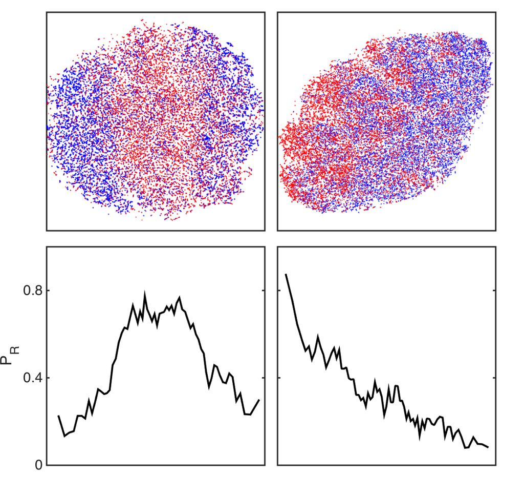
94 a b P (S R) P (S) S 6B;m`2 8Xd, h?2 +? ` +i2`bbib+b Q7 i?2 bq7im2bb }2H/X - bm Tb?Qi Q7 i?2 bvbi2k i T = 0.47 M/ ρ = 1.20 rbi? T `ib+h2b +QHQ`2/ ++Q`/BM; iq i?2b` bq7im2bb 7`QK `2/ UbQ7iV iq #Hm2 U? `/VX #- h?2 /Bbi`B#miBQM Q7 bq7im2bb Q7 HH T `ib+h2b BM i?2 bvbi2k U#H +FV M/ Q7 i?qb2 T `ib+h2b i? i `2 #Qmi `2 `` M;2 U`2/VX NyW Q7 i?2 T `ib+h2b i? i `2 #Qmi iq `2 `` M;2? p2 S > 0 Ub? /2/ `2;BQMVX LQM2 Q7 i?2 / i BM+Hm/2/ BM i?bb THQi r2`2 BM i?2 i` BMBM; b2ix? p2 bi`m+im`2 i? i Bb KQ`2 bbkbh ` iq?b;?2`@i2kt2` im`2 HB[mB/- r?2`2 i?2`2 `2 KQ`2 `2 `` M;2K2Mib- r?bh2? `/ T `ib+h2b r?qb2 bi`m+im`2 TT2 `b +HQb2` iq HQr2`@ i2kt2` im`2 HB[mB/ R38 X 6B;X R U V Bb bm Tb?Qi rbi? T `ib+h2b +QHQ`2/ ++Q`/BM; iq i?2b` bq7im2bbx 1pB@ /2MiHv- S? b bi`qm; bt ib H +Q``2H ibqmbx 6B;X R U#V b?qrb i?2 /Bbi`B#miBQM Q7 bq7im2bbp (S)- M/ i?2 /Bbi`B#miBQM Q7 bq7im2bb 7Q` T `ib+h2b Dmbi #27Q`2 i?2v ;Q i?`qm;? `2@ `` M;2K2Mi- P (S R)X q2 b22 i? i NyW Q7 i?2 T `ib+h2b i? i mm/2`;q `2 `` M;2K2Mib? p2 S > 0X q2? p2 HbQ i2bi2/ Qi?2` b2ib Q7 bi`m+im`2 7mM+iBQMb Ub22 bmtth2k2mi H BM7Q`K ibqmv M/ 7QmM/ M2 `Hv B/2MiB+ H ++m` +vx aq7im2bb Bb i?2`27q`2?b;?hv +@ +m` i2 T`2/B+iQ` Q7 `2 `` M;2K2Mib i? i Bb `2 bqm #Hv `Q#mbi iq i?2 b2i Q7 bi`m+im`2 7mM+iBQMb +?Qb2MX q2 M2ti b?qr i? i i?2 T`Q# #BHBiv i? i T `ib+h2b `2 `` M;2 Bb 7mM+iBQM Q7 i?2b` bq7im2bbx h?bb T`Q# #BHBiv Bb + H+mH i2/ b i?2 7` +ibqm Q7 T `ib+h2b Q7 bq7im2bb- S- dk

95 P R (S) P R (S) T =0.47 T =0.58 T P R (S) S = 3 S =3 P R (S) 1/T S P R (S) =P 0 (S)exp( E(S)/T ) P 0 (S) E(S) S P R (S)/P 0 (S) E(S)/T E(S) E(S) Σ(S) ln P 0 (S) S S E = e 0 e 1 S Σ=Σ 0 Σ 1 S T P R (S) T 0 Σ E/T 0 T 0 = e 1 /Σ 1 P R (S) T 0 T 0 T m 0 T 0 T = T 0

96 a c log PR S E S b d log PR T log (PR/P0) E/T /T T0 m P R (S) T = P R (S) dq(s, t)/dt T =0.47 T =0.58 P R (S) 1/T S 3 S 3 P R /P 0 E/T E Σ P R (S) =exp(σ E/T ) S T 0 T0 m ρ =1.15, 1.20, 1.25, 1.30 T 0 = T0 m

97 a b q(t) t/ t/ T = P R (S) q(t) = 1 N Θ( r i (t) r i (0) a) i N r i i Θ a =0.5 ρ = 1.20 q(t) P R (S) S t = 0 q(s, t) q(t) = dsq(s, t)p (S) q(s, t) S t dq(s,t) dt t=0 = c a P R (S) c a a dq(s,t) dt t=0 P R (S)

98 a G(S, 3,t) log (t/ ) S b G(S, 3,t) S c hs(t)is t/ S 0 3 t =0 t = 1000τ S 0 3 S 0 3 P R (S) q(s, t) S t 1 t (1 P R (S)) t 1 P R (S) q(t) q(t) G(S, S 0,t) t S 0 t =0 a t

99 t G(S, S 0 = 3,t) G(S, S 0,t) S 0 t t G(S, S 0 = 3,t) S(t) S0 = dssg(s, S 0,t) S 0 S 0 τ α G(S, S 0,t) = δ(s S 0 ) P R (S) q(s, t) G(S, S 0,t) S S 0 t q(t) r d 1 g(r) δ 0

100 g(r) R G X (i; r, δ) = j X e 1 2δ 2 (r R ij) 2 R ij i j X r σ AA 0.1σ AA Ψ XY (i; ξ,λ,ζ) = j X e (R2 ij +R2 jk +R2 ik )/ξ2 (1 + λ cos θ ijk ) ζ k Y θ ijk R ij R ik λ = ±1 ζ X Y G X (i; r, δ) X δ r

101 Structure"function"parameters"for"Ψ YZ ξ"(σ AA ) ζ λ g(r) g AB (r)

102 0.66 Type A 0.62 Accuracy r/σ Type B Accuracy r/σ r g AA (r)

103 Type A (r/ ) Type B (r/ ) Type A (r/ ) Type B (r/ ) 0.9σ AA 1.1σ AA

104 300 Type A Histogram Histogram r/σ Type B r/σ 1.9σ AA 1.1σ AA 0.8, σ AA

105 median weight r/σ AA N s = 15 N s N s = 15

106 Accuracy No. of structure functions S i = α w α G(i; rα,δ) w α r α G = (G G )/ δg 2 G(i; r, δ) r

107 wa rês AA wb rês AA r/σ AA g(r) g(r) g AA (r) g AB (r)

108 0.2 Type A neighbors 0.4 Type B neighbors gaa(r) g(r) AA H g H g - AA S g S g g AB H g g H - AB S g S g(r) gab(r) r/σ AA r/σ AA g H AX gs AX gax H gax S g AX(r) g AX (r)

109 i G Y cdf (i; µ) = j 1, R ij <µ. G Y cdf (i; µ) Y µ i Y µ σ AA 0.1σ AA Y lm ( r ) ( 4π Q l (i; r min,r max )= 2l +1 l m= l Q lm ( r ) 2 ) 1/2,

110 Q lm ( r ) = 1 Y lm ( R N ij ), r min <R ij <r max. j j Q lm ( r ) Y lm ( r ) j i Q l (i; r min,r max ) Q lm r min r max 0.5σ AA σ AA l l {2, 4, 6, 8, 10, 12, 14} ρ =1.15 T =0.37 ρ =1.2 T =0.47 g(r) Q l 2% G Y cdf Q l A B ( l ) 3/2 Ŵ l = W l Q lm ( r ) 2, m= l

111 W l = m 1,m 2,m 3 l l l m 1 m 2 m 3 ( Q lm1 ( r ) Q lm2 ( r ) Q lm3 ( r ) ) l l l m 1 m 2 m 3 3j W l l Q l P R P R (S) q(s, t) = 1 Θ( r i (t) r i (0) a)δ(s i (0) S) N S i

112 N S S t =0 t τ R (T ) P R (S) a P R (S) c(t )P R (S) c(t ) a c(t ) = c a f rrev (T ) c a a f rrev (T ) G(S, S 0,t) S 0 t =0 t f t = dsg(s, S 0,t)P R (S). t 1 t t 1 P (t S 0 )= (1 f t )f t = t =0 t 1 t =0 [ ] dsg(s, S 0,t )(1 P R (S)) dsg(s, S 0,t)P R (S) t

113 Q7 i?2 Qp2`H T 7mM+iBQM Ĝ rbhh #2 ;Bp2M #vt t< 1 #"! q(s0, t) = 1 t =0 t =0 dsg(s, S0, t )(1 PR (S)) $" dsg(s, S0, t )PR (S). U8XRdV h?bb ;Bp2b bq7im2bb /2T2M/2Mi T`2/B+iBQM 7Q` i?2 Qp2`H T i? i + M #2 +QKTmi2/ M@ HviB+ HHv QM+2 PR (S) M/ G(S, S0, t) `2 FMQrMX h?2 Qp2` HH Qp2`H T Bb `2H i2/ iq q(s, t) #v q(t) = " U8XR3V dsq(s, t)p (S). AM 6B;X 8XR3 U V r2 b22 i?2 Qp2`H T b 7mM+iBQM Q7 ibk2 7Q` /Bz2`2Mi bq7im2bb2b i irq `2T`2b2Mi ibp2 i2kt2` im`2bx AM #Qi? + b2b r2 b22 ;QQ/ ;`22K2Mi #2ir22M i?2 T`2@ /B+i2/ M/ K2 bm`2/ p Hm2b Q7 q(s, t)x abkbh `Hv BM 6B;X 8XR3 U#V r2 b22 i?2 p2` ; qhtl <qhs,tl> Qp2`H T 7Q` HH i2kt2` im`2b +QMbB/2`2/ M/ }M/ bbkbh `Hv ;QQ/ ;`22K2MiX têt têt B;m`2 8XR3, h?2 MQM@2tTQM2MiB H /2+ v Q7 Qp2`H TX U V i?2 bq7im2bb@/2t2m/2mi Qp2`H T q(s, t) 7Q` irq `2T`2b2Mi ibp2 i2kt2` im`2b T = 0.47 UHQM; ibk2v M/ T = 0.58 Ub?Q`i ibk2v i 7Qm` bq7im2bb2b 7`QK 4 U#Hm2V iq 4 U`2/VX U#V i?2 p2` ;2 Qp2`H T i HH i2kt2` im`2b 7`QK T = 0.45 U#Hm2V iq T = 0.70 U`2/VX q?2m +QKTmiBM; q(s, t) r2 TT`QtBK i2 G(S, S0, t) #v : mbbb M #2+ mb2 Bi HHQrb mb iq +QMpQHp2 i?2 T`Q# #BHBiv Q7 `2 `` M;2K2Mi- PR (S)- rbi? i?2 T`QT ; iq` M Hvi@ NR

114 G(S, S 0,t) P R (S) G(S, S 0,t) q(s, t) P (S) q(t) q(t) =1 t t =0 [ t 1 t =0 ds(1 P R (S))P (S, t )] dsp R (S)P (S, t ) P (S, t) = ds 0 G(S, S 0,t)P(S 0 ) P (S, t) t P (S, t) q(s, t) γ C

115 Accuracy Gamma C γ E log P 0 S

116 P R (S) P R (S) 1 DE ÊÊ ÊÊÊ Ê Ê Ê Ê Ê ÊÊ ÊÊ ÊÊÊÊ Ê ÊÊÊÊ Ê ÊÊÊÊ Ê Ê Ê ÊÊÊÊ Ê ÊÊÊÊÊ S E(S) S T =0.47 ρ =1.20 Ê E(S) log P 0 (S) S E(S) =E 0 + E 1 S + E 2 S 2 E 2 E 1 a =0.5

117 t =0 τ R (T ) a b =0.2 b f rrev f rrev f rrev f rrev firrev S X firrev\ T f rrev T =0.47 T =0.63

118 T 0 T 0

119 6

120

121

122 σ AA ϵ AA m kt/ϵ =0.1 γ = 10 4 kt/ϵ =0.47 ρ =1.2 d =3 τ τ = mσaa 2 /ϵ AA 2τ p p t t A =[t t/2,t] B =[t, t + t/2] p (t) = (r i r i B ) 2 A (r i r i A ) 2 B

123 A B A B r i A = r i B p p p >p c =0.2 p i D 2 (i) = j R ij <R c [R ij (t + t) Λ R ij (t)] 2 Λ R c =2.5σ t =5τ D 2 S [ P R (S) =exp Σ(S) E(S) ] kt Σ(S) =Σ 0 Σ 1 S E(S) =e 0 e 1 S

124 i Σ(S) E(S) T 0 d =3 G X (i; r, σ) = 1 2π j X e 1 2σ 2 (R ij r) 2 R ij i j r ± σ i g(r) r

125 d =3 σ AA (a) (b)

126 E L > 18 E L > (a) (b) (c) PR(NC) 10-3 PR(EL) 10-3 PR(S) N C E L S 10 6 i X i X P R (X i ) X i

127 X i µ X σ X X i X i Q = P R(X i >µ X + σ X ) P R (X i <µ X σ X ) X i X i X X Q = 6.2 Q =5.0 Q = 165 Q Q 20 Q Q T =0.35. Q 500 Q =7.6 Q =9.9 Q

128 g(r) r

129 N T N O P R (S)

130 10 0 h A(0) A(r)i r/ ξ =1.2 ξ =1.1 δs i = S i S (S S ) 2. δs(0)δs(r) r δs(0)δs(r) = Ae r/ξ. ξ 1.2

131 p δp(0)δp(r) ξ 1.1 i (S j S i )R ij S i = R 2. j R ij <R c ij R c =2.5σ AA α i t α t α r iα = r i (t α ) r i (t α ). i cos θ = r S r S. cos θ r S

132 r S (a) (b) 0 apple r rs < 1 1 apple r rs < 2 2 apple r rs < 3 3 apple r rs < 4 hcos i P (cos ) rs r cos i r i S i r S P (cos θ) r S cos θ r S cos θ r S r S r S r S 60 deg S cos θ r S r S

133 d =3 w b G i i S i = w G i + b w α w b = 0 G iµ = G(i; µσ, σ) µ r µ = µσ R c N σ = R c /σ w(r µ ) w µ N σ S i = w(r µ )G(i; r µ,σ). µ=0

134 waa(r) wab(r) (a) (b) gaa(r) gab(r) (c) (d) r/ g AA (r) g AB (r) σ 0 r = r µ = µσ N σ lim σ = σ 0 µ=0 lim σ 0 Rc 0 dr 1 2πσ e 1 2σ 2 r2 = δ(r) S i = Rc 0 dr j δ(r ij r) w(r). r

135 i S i = j w(r ij) 82.5% 88% S i = j A A AA e α AAR ij + j B A AB e α ABR ij. r<σ HS σ HS C XY w XY (r) = A XY e α XY r r<σ HS XY r>σ HS XY.

136 85% M R M

137 d =2 d =3 0.3σ AA

138 0.3σ AA 2.5σ AA d =2 d =2 d =3 d =2 d =3 d =2 d =2 d =3

139

140

141

142

143

144

145

146

147

148

149

150

151

152

153

154

155

156

157 β

158

159

160