Hartree-Fock Theory. Solving electronic structure problem on computers
|
|
|
- Αριάδνη Τρικούπη
- 7 χρόνια πριν
- Προβολές:
Transcript
1
2 Hartree-Foc Theory Solving electronic structure problem on computers Hartree product of non-interacting electrons mean field molecular orbitals expectations values one and two electron operators Pauli Principle slater determinant of molecular orbitals expectations values of one and two electron operators energy of slater determinant variation principle optimizing the orbitals in slater determinant one-particle mean-field foc operator self-consistent-field linear combinations atomic orbitals & basissets Roothaan Hall equations
3 Hartree-Foc Theory for n electrons mean-field approach H = i atomic units 2 2m e 2 i A e 2 Z A 4π 0 r i R A + vmf i (r i ) h i (r i )= 2 i + A independent electrons H = h i (r i ) i Z A r ia + v mf i (r i ) one-electron wavefunctions (molecular orbitals) h i (r) i (r) = i i (r) orthonormal i (r) j (r)dr = δ ij Hartree product of n distinghuisable electrons Ψ(r 1, r 2,...,r n )= 1 (r 1 ) 2 (r 2 )... n (r n )
4 Hartree-Foc Theory for n electrons indistinguishable electrons fermions with 3 spatial and 1 spin coordinate (4D) {x} = {r,s} Pauli principle Ψ(r 1, x 2,..,x i, x j,...,x n )= Ψ(x 1, x 2,..,x j, x i,...,x n ) spin orbitals ϕ i (x) = i (r)α(s) i (r)β(s) spin functions α(s)β(s)ds = δ αβ
5 Hartree-Foc Theory for n electrons anitsymmetric linear combination of Hartree products: i.e. 2 electrons Ψ(x 1, x 2 )= 1 2 [ϕ 1 (x 1 )ϕ 2 (x 2 ) ϕ 2 (x 1 )ϕ 1 (x 2 )] n electrons: Slater determinant Ψ(x 1, x 2,..,x n )= 1 n ϕ 1 (x 1 ) ϕ 1 (x 2 ).. ϕ 1 (x n ) ϕ 2 (x 1 ) ϕ 2 (x 2 ).. ϕ 2 (x n ) ϕ n (x 1 ) ϕ n (x 2 ).. ϕ n (x n )
6 Hartree-Foc Theory for n electrons anitsymmetric linear combination of Hartree products: i.e. 2 electrons Ψ(x 1, x 2 )= 1 2 [ϕ 1 (x 1 )ϕ 2 (x 2 ) ϕ 2 (x 1 )ϕ 1 (x 2 )] n electrons: Slater determinant Ψ(x 1, x 2,..,x n )= 1 n ϕ 1 (x 1 ) ϕ 1 (x 2 ).. ϕ 1 (x n ) ϕ 2 (x 1 ) ϕ 2 (x 2 ).. ϕ 2 (x n ) ϕ n (x 1 ) ϕ n (x 2 ).. ϕ n (x n )
7 Hartree-Foc Theory for n electrons Expectations values for one and two electron operators Hartree product (no spin) Ô1 = a a (x 1 )ô(r 1 ) a (r 1 )dr 1 Ô2 = 1 2 a b a (r 1 ) b (r 2)ô(r 1, r 2 ) a (r 1 ) b (r 2 )dr 1 dr 2 Slater determinant (spin, Pauli principle) Ô1 = a a (x 1 )ô(r 1 ) a (x 1 )dx 1 Ô2 = a a b a (x 1 ) b (x 2)ô(r 1, r 2 ) a (x 1 ) b (x 2 )dx 1 dx 2 b a (x 1 ) b (x 2)ô(r 1, r 2 ) b (x 1 ) a (x 2 )dx 1 dx 2 Ô2 = 1 2 a b a (x 1 ) b (x 2)ô(r 1, r 2 )(1 ˆp 12 ) a (x 1 ) b (x 2 )dx 1 dx 2
8 Wassermoleül 2 H + 1 O Eletronen 10 Moleülorbitale

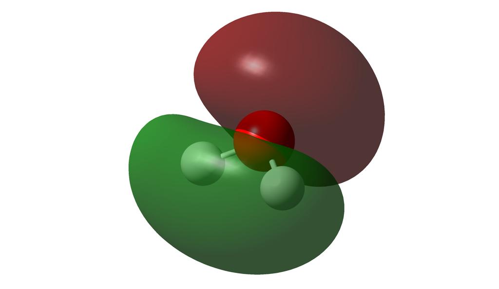
9 Wassermoleül 2 H+ 1 O8+ 10 Eletronen 10 Moleülorbitale
10 2 H+ 1 O8+ 10 Eletronen 10 Moleülorbitale Energie Wassermoleül


11 Hartree-Foc theory mean field approach vary orbitals until until self-consistency (SCF)
12 Hartree-Foc Theory for n electrons Hartree-Foc eigenvalue equations ˆf(x 1 )ϕ i (r 1 )= i ϕ(r 1 ) solving non-linear eigenvalues equations numerically step 1: get rid of spin and express in real spatial orbitals step 2: expand spatial orbitals in basis functions restricted Hartree Foc electron pair with opposite spin in same spatial orbital ϕ i (x) = j (r)α(s) ϕ i+1 (x) = j (r)β(s)
13 Hartree-Foc Theory for n electrons solving non-linear eigenvalues equations numerically step 1: get rid of spin and express in real spatial orbitals ˆf(x 1 ) i (r 1 )α(s 1 ) = ĥ0 (r 1 ) i (r 1 )α(s 1 ) + n/2 + n/2 n/2 n/2 (r 2 )α (s 2 ) 1 (r 2 )α(s 2 ) i (r 1 )α(s 1 )dr 2 ds 2 (r 2 )β (s 2 ) 1 (r 2 )β(s 2 ) i (r 1 )α(s 1 )dr 2 ds 2 (r 2 )α (s 2 ) 1 i (r 2 )α(s 2 ) (r 1 )α(s 1 )dr 2 ds 2 (r 2 )β (s 2 ) 1 i (r 2 )α(s 2 ) (r 1 )β(s 1 )dr 2 ds 2
14 Hartree-Foc Theory for n electrons solving non-linear eigenvalues equations numerically step 1: get rid of spin and express in real spatial orbitals ˆf(x 1 ) i (r 1 )α(s 1 ) = ĥ0 (r 1 ) i (r 1 )α(s 1 ) + n/2 + n/2 n/2 n/2 (r 2 )α (s 2 ) 1 (r 2 )α(s 2 ) i (r 1 )α(s 1 )dr 2 ds 2 (r 2 )β (s 2 ) 1 (r 2 )β(s 2 ) i (r 1 )α(s 1 )dr 2 ds 2 (r 2 )α (s 2 ) 1 i (r 2 )α(s 2 ) (r 1 )α(s 1 )dr 2 ds 2 (r 2 )β (s 2 ) 1 i (r 2 )α(s 2 ) (r 1 )β(s 1 )dr 2 ds 2
15 Hartree-Foc Theory for n electrons solving non-linear eigenvalues equations numerically step 1: get rid of spin and express in real spatial orbitals ˆf(x 1 ) i (r 1 )α(s 1 ) = ĥ0 (r 1 ) i (r 1 )α(s 1 ) + n/2 + n/2 n/2 (r 2 ) 1 (r 2 ) i (r 1 )α(s 1 )dr 2 (r 2 ) 1 (r 2 ) i (r 1 )α(s 1 )dr 2 (r 2 ) 1 i (r 2 ) (r 1 )α(s 1 )dr 2
16 Hartree-Foc Theory for n electrons solving non-linear eigenvalues equations numerically step 1: get rid of spin and express in real spatial orbitals α (s 1 ) ˆf(x 1 )α(s 1 )ds 1 i (r 1 ) = α (s 1 )ĥ0 (r 1 )(r 1 )α(s 1 )ds 1 + n/2 + n/2 n/2 α (s 1 ) (r 2) 1 (r 2 ) i (r 1 )α(s 1 )dr 2 ds 1 α (s 1 ) (r 2) 1 (r 2 ) i (r 1 )α(s 1 )dr 2 ds 1 α (s 1 ) (r 2) 1 i (r 2 ) (r 1 )α(s 1 )dr 2 ds 1 Hartree-Foc eigenvalue equation for spatial orbitals ˆf(r 1 ) i (r 1 ) = ĥ0 (r 1 )(r 1 ) +2 n/2 (r 2 ) 1 (r 2 ) i (r 1 )dr 2 n/2 (r 2 ) 1 i (r 2 ) (r 1 )dr = i i (r 1 )
17 Hartree-Foc Theory for n electrons solving non-linear eigenvalues equations numerically step 1: get rid of spin and express in real spatial orbitals ˆf(r 1 ) i (r 1 ) = ĥ0 (r 1 )(r 1 ) +2 n/2 (r 2 ) 1 (r 2 ) i (r 1 )dr 2 n/2 (r 2 ) 1 i (r 2 ) (r 1 )dr = i i (r 1 ) step 2: expand spatial orbitals in basis functions (basisset) i (r) = j c ij γ j (r R j )
18 Hartree-Foc Theory for n electrons linear combination of atomic orbitals i (r) = j c ij γ j (r R j ) hydrogen-lie orbitals (one possibility out of many...) γ 1 = ψ 1s (ζ 1 ) γ 2 = ψ 2s (ζ 2 ) γ 3 = ψ 2p (ζ 3 ) γ 4 =...


19 Wasserstoffmoleül Lineare Kombination von einzelne Wasserstoff-Orbitale - = 2(1 + S12 ) atomorbital moleülorbital + = 2(1 + S12 )
20 Hartree-Foc Theory for n electrons solving non-linear eigenvalues equations numerically step 2: expand spatial orbitals in basis functions ˆf(r 1 ) i (r 1 )= i i (r 1 ) i (r) = j c ij γ j (r R j ) ν ˆf(r 1 ) ν c νi γ ν (r 1 )= i c νi γ ν (r 1 ) c νi γµ(r 1 ) ˆf(r 1 )γ ν (r 1 )dr 1 = i c νi ν ν γ µ (r 1 )γ ν (r 1 )dr 1
21 Hartree-Foc Theory for n electrons solving non-linear eigenvalues equations numerically step 2: expand spatial orbitals in basis functions (basisset) c νi γµ(r 1 ) ˆf(r 1 )γ ν (r 1 )dr 1 = i c νi ν ν γ µ (r 1 )γ ν (r 1 )dr 1 express in terms of matrices F µν c νi = i ν ν S µν c νi solution if, and only if FC = SC F i S =0
22 Hartree-Foc Theory for n electrons solving non-linear eigenvalues equations numerically non-linear: F depends on C F µν = γ µ(r 1 )ĥ0 (r 1 )γ ν (r 1 )dr 1 +2 a γ µ (r 1 ) a(r 2 ) 1 a (r 2 )γ ν (r 1 )dr 1 dr a γ µ (r 1 ) a(r 2 ) 1 γ ν (r 2 ) a (r 1 )dr 1 dr F µν = h 0 µν +2 a a κ κ λ c κac λa λ c κac λa γ µ (r 1 )γ κ(r 2 ) 1 γ λ (r 2 )γ ν (r 1 )dr 1 dr γ µ (r 1 )γ κ(r 2 ) 1 γ ν (r 2 )γ a (r 1 )dr 1 dr

23 Hartree-Foc Roothaan-Hall equations non-linear eigenvalue problem Fc = i Sc practical algorithm iterate until self-consistency pre-compute integrals of basisset F µν = γ µ ˆf γ ν S µν = γ µ γ ν
24 Basissets minimal basis (1 function per shell) H-He: 1s (1) Li-Ne: 1s, 2s, 2px, 2py, 2pz (5) Na-Ar: 1s, 2s, 2px, 2py, 2pz, 3s, 3px, 3py, 3pz (9) Slater-type orbitals computationally demanding f 1s (ζ, r) =exp[ ζr] Gaussian-type orbitals computationally convenient g 1s (α, r) = (8α 3 /π 3 ) 1/4 exp[ αr 2 ] g (α, r) 2px = (128α 5 /π 3 ) 1/4 x exp[ αr 2 ] g (α, r) 3dxy = (2048α 7 /π 3 ) 1/4 xy exp[ αr 2 ]
25 Basissets Gaussian-type orbitals computationally convenient, but not as accurate as Slater-type orbitals linear combination (contraction) of several gaussians (primitives) STO-3G CGF 1s = 3 i d i,1sg 1s (α i,1s ) CGF 2s = 3 i d i,2sg 1s (α i,2sp ) CGF 2p = 3 i d i,2pg 2p (α i,2sp ) least-square fit to Slater orbitals min SF 1s (r) CGF 1s (r))dr] 2 min SF 2s (r) CGF 2s (r) dr SF 2p (r) CGF 2p (r) dr 2
26 Basissets Double-Zeta basis two basisfunctions (contractions) per valence orbital 3-21G, 4-31G, 6-31G H-He: 1s = 2 i d i,1sg 1s (α i,1s ) 1s = g 1s (α i,1s ) Li-Ne: 1s = 3 i d i,1sg 1s (α i,1s ) 2s = 2 i d i,2s g 1s(α i,2sp ) 2s = g 1s (α i,2sp ) 2p = 2 i d i,2p g 2p(α i,2sp ) 2p = g 2p (α i,2sp )
27 Basissets Double-Zeta basis with polarization functions two basisfunctions (contractions) per valence orbital Li-Ne: 3d functions (*) H-He: 2p functions (**) 3-21G*, 4-31G*, 6-31G*, 6-31G**
Solutions to the Schrodinger equation atomic orbitals. Ψ 1 s Ψ 2 s Ψ 2 px Ψ 2 py Ψ 2 pz
 Solutions to the Schrodinger equation atomic orbitals Ψ 1 s Ψ 2 s Ψ 2 px Ψ 2 py Ψ 2 pz ybridization Valence Bond Approach to bonding sp 3 (Ψ 2 s + Ψ 2 px + Ψ 2 py + Ψ 2 pz) sp 2 (Ψ 2 s + Ψ 2 px + Ψ 2 py)
Review: Molecules = + + = + + Start with the full Hamiltonian. Use the Born-Oppenheimer approximation
 Review: Molecules Start with the full amiltonian Ze e = + + ZZe A A B i A i me A ma ia, 4πε 0riA i< j4πε 0rij A< B4πε 0rAB Use the Born-Oppenheimer approximation elec Ze e = + + A A B i i me ia, 4πε 0riA
ψ ( 1,2,...N ) = Aϕ ˆ σ j σ i χ j ψ ( 1,2,!N ) ψ ( 1,2,!N ) = 1 General Equations
 = Aϕ ˆ σ j σ i χ j ψ ( 1,2,!N ) ψ ( 1,2,!N ) = 1 General Equations") General Equations Our goal is to construct the best single determinant wave function for a system of electrons. By best we mean the determinant having the lowest energy. We write our trial function as
General Equations Our goal is to construct the best single determinant wave function for a system of electrons. By best we mean the determinant having the lowest energy. We write our trial function as
The Hartree-Fock Equations
 he Hartree-Fock Equations Our goal is to construct the best single determinant wave function for a system of electrons. We write our trial function as a determinant of spin orbitals = A ψ,,... ϕ ϕ ϕ, where
Variational Wavefunction for the Helium Atom
 Technische Universität Graz Institut für Festkörperphysik Student project Variational Wavefunction for the Helium Atom Molecular and Solid State Physics 53. submitted on: 3. November 9 by: Markus Krammer
Τίτλος: Eνεργά δυναμικά στη θεωρία συναρτησιακών του πρώτου πίνακα πυκνότητας
 Τίτλος: Eνεργά δυναμικά στη θεωρία συναρτησιακών του πρώτου πίνακα πυκνότητας Μπουσιάδη Σοφία Τριμελής επιτροπή: Ν. Λαθιωτάκης (Ε.Ι.Ε) Ι. Λελίδης (Ε.Κ.Π.Α) Ι. Πετσαλάκης (Ε.Ι.Ε) Περιεχόμενα Εισαγωγή στην
Phys460.nb Solution for the t-dependent Schrodinger s equation How did we find the solution? (not required)
") Phys460.nb 81 ψ n (t) is still the (same) eigenstate of H But for tdependent H. The answer is NO. 5.5.5. Solution for the tdependent Schrodinger s equation If we assume that at time t 0, the electron starts
Phys460.nb 81 ψ n (t) is still the (same) eigenstate of H But for tdependent H. The answer is NO. 5.5.5. Solution for the tdependent Schrodinger s equation If we assume that at time t 0, the electron starts
Lecture 2: Dirac notation and a review of linear algebra Read Sakurai chapter 1, Baym chatper 3
 Lecture 2: Dirac notation and a review of linear algebra Read Sakurai chapter 1, Baym chatper 3 1 State vector space and the dual space Space of wavefunctions The space of wavefunctions is the set of all
Matrices and Determinants
 Matrices and Determinants SUBJECTIVE PROBLEMS: Q 1. For what value of k do the following system of equations possess a non-trivial (i.e., not all zero) solution over the set of rationals Q? x + ky + 3z
6.1. Dirac Equation. Hamiltonian. Dirac Eq.
 6.1. Dirac Equation Ref: M.Kaku, Quantum Field Theory, Oxford Univ Press (1993) η μν = η μν = diag(1, -1, -1, -1) p 0 = p 0 p = p i = -p i p μ p μ = p 0 p 0 + p i p i = E c 2 - p 2 = (m c) 2 H = c p 2
Numerical Analysis FMN011
 Numerical Analysis FMN011 Carmen Arévalo Lund University carmen@maths.lth.se Lecture 12 Periodic data A function g has period P if g(x + P ) = g(x) Model: Trigonometric polynomial of order M T M (x) =
Problem Set 9 Solutions. θ + 1. θ 2 + cotθ ( ) sinθ e iφ is an eigenfunction of the ˆ L 2 operator. / θ 2. φ 2. sin 2 θ φ 2. ( ) = e iφ. = e iφ cosθ.
 sinθ e iφ is an eigenfunction of the ˆ L 2 operator. / θ 2. φ 2. sin 2 θ φ 2. ( ) = e iφ. = e iφ cosθ.") Chemistry 362 Dr Jean M Standard Problem Set 9 Solutions The ˆ L 2 operator is defined as Verify that the angular wavefunction Y θ,φ) Also verify that the eigenvalue is given by 2! 2 & L ˆ 2! 2 2 θ 2 +
Chemistry 362 Dr Jean M Standard Problem Set 9 Solutions The ˆ L 2 operator is defined as Verify that the angular wavefunction Y θ,φ) Also verify that the eigenvalue is given by 2! 2 & L ˆ 2! 2 2 θ 2 +
Αρχές Κβαντικής Χημείας και Φασματοσκοπίας
 ΑΡΙΣΤΟΤΕΛΕΙΟ ΠΑΝΕΠΙΣΤΗΜΙΟ ΘΕΣΣΑΛΟΝΙΚΗΣ ΑΝΟΙΚΤΑ ΑΚΑΔΗΜΑΪΚΑ ΜΑΘΗΜΑΤΑ Αρχές Κβαντικής Χημείας και Φασματοσκοπίας Ενότητα # (6): LCAO - Εξισώσεις Roothaan-Hartree-Fock - Αυτοσυνεπές πεδίο Καραφίλογλου Παντελεήμων
( ) 2 and compare to M.
 2 and compare to M.") Problems and Solutions for Section 4.2 4.9 through 4.33) 4.9 Calculate the square root of the matrix 3!0 M!0 8 Hint: Let M / 2 a!b ; calculate M / 2!b c ) 2 and compare to M. Solution: Given: 3!0 M!0 8
Problems and Solutions for Section 4.2 4.9 through 4.33) 4.9 Calculate the square root of the matrix 3!0 M!0 8 Hint: Let M / 2 a!b ; calculate M / 2!b c ) 2 and compare to M. Solution: Given: 3!0 M!0 8
( ) = a(1)b( 2 ) c( N ) is a product of N orthonormal spatial
 = a(1)b( 2 ) c( N ) is a product of N orthonormal spatial") Many Electron Spin Eigenfunctions An arbitrary Slater determinant for N electrons can be written as ÂΦ,,,N )χ M,,,N ) Where Φ,,,N functions and χ M ) = a)b ) c N ) is a product of N orthonormal spatial,,,n
Many Electron Spin Eigenfunctions An arbitrary Slater determinant for N electrons can be written as ÂΦ,,,N )χ M,,,N ) Where Φ,,,N functions and χ M ) = a)b ) c N ) is a product of N orthonormal spatial,,,n
Electronic structure and spectroscopy of HBr and HBr +
 Electronic structure and spectroscopy of HBr and HBr + Gabriel J. Vázquez 1 H. P. Liebermann 2 H. Lefebvre Brion 3 1 Universidad Nacional Autónoma de México Cuernavaca México 2 Universität Wuppertal Wuppertal
Jesse Maassen and Mark Lundstrom Purdue University November 25, 2013
 Notes on Average Scattering imes and Hall Factors Jesse Maassen and Mar Lundstrom Purdue University November 5, 13 I. Introduction 1 II. Solution of the BE 1 III. Exercises: Woring out average scattering
Srednicki Chapter 55
 Srednicki Chapter 55 QFT Problems & Solutions A. George August 3, 03 Srednicki 55.. Use equations 55.3-55.0 and A i, A j ] = Π i, Π j ] = 0 (at equal times) to verify equations 55.-55.3. This is our third
Quadratic Expressions
 Quadratic Expressions. The standard form of a quadratic equation is ax + bx + c = 0 where a, b, c R and a 0. The roots of ax + bx + c = 0 are b ± b a 4ac. 3. For the equation ax +bx+c = 0, sum of the roots
Chapter 6: Systems of Linear Differential. be continuous functions on the interval
 Chapter 6: Systems of Linear Differential Equations Let a (t), a 2 (t),..., a nn (t), b (t), b 2 (t),..., b n (t) be continuous functions on the interval I. The system of n first-order differential equations
SCHOOL OF MATHEMATICAL SCIENCES G11LMA Linear Mathematics Examination Solutions
 SCHOOL OF MATHEMATICAL SCIENCES GLMA Linear Mathematics 00- Examination Solutions. (a) i. ( + 5i)( i) = (6 + 5) + (5 )i = + i. Real part is, imaginary part is. (b) ii. + 5i i ( + 5i)( + i) = ( i)( + i)
Concrete Mathematics Exercises from 30 September 2016
 Concrete Mathematics Exercises from 30 September 2016 Silvio Capobianco Exercise 1.7 Let H(n) = J(n + 1) J(n). Equation (1.8) tells us that H(2n) = 2, and H(2n+1) = J(2n+2) J(2n+1) = (2J(n+1) 1) (2J(n)+1)
Exercises 10. Find a fundamental matrix of the given system of equations. Also find the fundamental matrix Φ(t) satisfying Φ(0) = I. 1.
 satisfying Φ(0) = I. 1.") Exercises 0 More exercises are available in Elementary Differential Equations. If you have a problem to solve any of them, feel free to come to office hour. Problem Find a fundamental matrix of the given
Exercises 0 More exercises are available in Elementary Differential Equations. If you have a problem to solve any of them, feel free to come to office hour. Problem Find a fundamental matrix of the given
Jordan Form of a Square Matrix
 Jordan Form of a Square Matrix Josh Engwer Texas Tech University josh.engwer@ttu.edu June 3 KEY CONCEPTS & DEFINITIONS: R Set of all real numbers C Set of all complex numbers = {a + bi : a b R and i =
1 String with massive end-points
 1 String with massive end-points Πρόβλημα 5.11:Θεωρείστε μια χορδή μήκους, τάσης T, με δύο σημειακά σωματίδια στα άκρα της, το ένα μάζας m, και το άλλο μάζας m. α) Μελετώντας την κίνηση των άκρων βρείτε
CHAPTER 48 APPLICATIONS OF MATRICES AND DETERMINANTS
 CHAPTER 48 APPLICATIONS OF MATRICES AND DETERMINANTS EXERCISE 01 Page 545 1. Use matrices to solve: 3x + 4y x + 5y + 7 3x + 4y x + 5y 7 Hence, 3 4 x 0 5 y 7 The inverse of 3 4 5 is: 1 5 4 1 5 4 15 8 3
Partial Differential Equations in Biology The boundary element method. March 26, 2013
 The boundary element method March 26, 203 Introduction and notation The problem: u = f in D R d u = ϕ in Γ D u n = g on Γ N, where D = Γ D Γ N, Γ D Γ N = (possibly, Γ D = [Neumann problem] or Γ N = [Dirichlet
Derivation of Quadratic Response Time Dependent Hartree-Fock (TDHF) Equations
 Equations") Derivation of Quadratic Response Time Dependent Hartree-Fock (TDHF) Equations Joshua Goings, Feizhi Ding, Xiaosong Li Department of Chemistry, University of Washington Nember 21, 2014 1 Derivation of Equations
Derivation of Quadratic Response Time Dependent Hartree-Fock (TDHF) Equations Joshua Goings, Feizhi Ding, Xiaosong Li Department of Chemistry, University of Washington Nember 21, 2014 1 Derivation of Equations
Œ ˆ Œ Ÿ Œˆ Ÿ ˆŸŒˆ Œˆ Ÿ ˆ œ, Ä ÞŒ Å Š ˆ ˆ Œ Œ ˆˆ
 ˆ ˆŠ Œ ˆ ˆ Œ ƒ Ÿ 018.. 49.. 4.. 907Ä917 Œ ˆ Œ Ÿ Œˆ Ÿ ˆŸŒˆ Œˆ Ÿ ˆ œ, Ä ÞŒ Å Š ˆ ˆ Œ Œ ˆˆ.. ³μ, ˆ. ˆ. Ë μ μ,.. ³ ʲ μ ± Ë ²Ó Ò Ö Ò Í É Å μ ± ÊÎ μ- ² μ É ²Ó ± É ÉÊÉ Ô± ³ É ²Ó μ Ë ±, μ, μ Ö μ ² Ìμ μé Ê Ö ±
Example Sheet 3 Solutions
 Example Sheet 3 Solutions. i Regular Sturm-Liouville. ii Singular Sturm-Liouville mixed boundary conditions. iii Not Sturm-Liouville ODE is not in Sturm-Liouville form. iv Regular Sturm-Liouville note
FORMULAS FOR STATISTICS 1
 FORMULAS FOR STATISTICS 1 X = 1 n Sample statistics X i or x = 1 n x i (sample mean) S 2 = 1 n 1 s 2 = 1 n 1 (X i X) 2 = 1 n 1 (x i x) 2 = 1 n 1 Xi 2 n n 1 X 2 x 2 i n n 1 x 2 or (sample variance) E(X)
Module 5. February 14, h 0min
 Module 5 Stationary Time Series Models Part 2 AR and ARMA Models and Their Properties Class notes for Statistics 451: Applied Time Series Iowa State University Copyright 2015 W. Q. Meeker. February 14,
3.4 SUM AND DIFFERENCE FORMULAS. NOTE: cos(α+β) cos α + cos β cos(α-β) cos α -cos β
 cos α + cos β cos(α-β) cos α -cos β") 3.4 SUM AND DIFFERENCE FORMULAS Page Theorem cos(αβ cos α cos β -sin α cos(α-β cos α cos β sin α NOTE: cos(αβ cos α cos β cos(α-β cos α -cos β Proof of cos(α-β cos α cos β sin α Let s use a unit circle
3.4 SUM AND DIFFERENCE FORMULAS Page Theorem cos(αβ cos α cos β -sin α cos(α-β cos α cos β sin α NOTE: cos(αβ cos α cos β cos(α-β cos α -cos β Proof of cos(α-β cos α cos β sin α Let s use a unit circle
General 2 2 PT -Symmetric Matrices and Jordan Blocks 1
 General 2 2 PT -Symmetric Matrices and Jordan Blocks 1 Qing-hai Wang National University of Singapore Quantum Physics with Non-Hermitian Operators Max-Planck-Institut für Physik komplexer Systeme Dresden,
Reminders: linear functions
 Reminders: linear functions Let U and V be vector spaces over the same field F. Definition A function f : U V is linear if for every u 1, u 2 U, f (u 1 + u 2 ) = f (u 1 ) + f (u 2 ), and for every u U
Math 6 SL Probability Distributions Practice Test Mark Scheme
 Math 6 SL Probability Distributions Practice Test Mark Scheme. (a) Note: Award A for vertical line to right of mean, A for shading to right of their vertical line. AA N (b) evidence of recognizing symmetry
Exercise 1.1. Verify that if we apply GS to the coordinate basis Gauss form ds 2 = E(u, v)du 2 + 2F (u, v)dudv + G(u, v)dv 2
du 2 + 2F (u, v)dudv + G(u, v)dv 2") Math 209 Riemannian Geometry Jeongmin Shon Problem. Let M 2 R 3 be embedded surface. Then the induced metric on M 2 is obtained by taking the standard inner product on R 3 and restricting it to the tangent
Math 209 Riemannian Geometry Jeongmin Shon Problem. Let M 2 R 3 be embedded surface. Then the induced metric on M 2 is obtained by taking the standard inner product on R 3 and restricting it to the tangent
6.3 Forecasting ARMA processes
 122 CHAPTER 6. ARMA MODELS 6.3 Forecasting ARMA processes The purpose of forecasting is to predict future values of a TS based on the data collected to the present. In this section we will discuss a linear
Chapter 6: Systems of Linear Differential. be continuous functions on the interval
 Chapter 6: Systems of Linear Differential Equations Let a (t), a 2 (t),..., a nn (t), b (t), b 2 (t),..., b n (t) be continuous functions on the interval I. The system of n first-order differential equations
Practice Exam 2. Conceptual Questions. 1. State a Basic identity and then verify it. (a) Identity: Solution: One identity is csc(θ) = 1
 Identity: Solution: One identity is csc(θ) = 1") Conceptual Questions. State a Basic identity and then verify it. a) Identity: Solution: One identity is cscθ) = sinθ) Practice Exam b) Verification: Solution: Given the point of intersection x, y) of the
Conceptual Questions. State a Basic identity and then verify it. a) Identity: Solution: One identity is cscθ) = sinθ) Practice Exam b) Verification: Solution: Given the point of intersection x, y) of the
EE512: Error Control Coding
 EE512: Error Control Coding Solution for Assignment on Finite Fields February 16, 2007 1. (a) Addition and Multiplication tables for GF (5) and GF (7) are shown in Tables 1 and 2. + 0 1 2 3 4 0 0 1 2 3
Η απωστική αυτή ενέργεια αίρει τον εκφυλισµό ως προς l σε σηµαντικό βαθµό. Αµελωντας το απωστικό δυναµικό, προκύπτει ενέργεια συνδεσης ίση µε
 Η άπωση ηλεκτρονίων και η αρχή του Πάουλι Για την ολική ενέργεια σύνδεσης πρέπει να ληφθεί υπόψη τόσο το δυνάµικό Κουλόµπ ενός εκάστου ηλεκτρονίου από τον πυρήνα καθώς και το απωστικό δυναµικό της αλληλεπίδρασης
If we restrict the domain of y = sin x to [ π, π ], the restrict function. y = sin x, π 2 x π 2
![If we restrict the domain of y = sin x to [ π, π ], the restrict function. y = sin x, π 2 x π 2](/thumbs/53/31933086.jpg "If we restrict the domain of y = sin x to [ π, π ], the restrict function. y = sin x, π 2 x π 2") Chapter 3. Analytic Trigonometry 3.1 The inverse sine, cosine, and tangent functions 1. Review: Inverse function (1) f 1 (f(x)) = x for every x in the domain of f and f(f 1 (x)) = x for every x in the
Chapter 3. Analytic Trigonometry 3.1 The inverse sine, cosine, and tangent functions 1. Review: Inverse function (1) f 1 (f(x)) = x for every x in the domain of f and f(f 1 (x)) = x for every x in the
4.6 Autoregressive Moving Average Model ARMA(1,1)
") 84 CHAPTER 4. STATIONARY TS MODELS 4.6 Autoregressive Moving Average Model ARMA(,) This section is an introduction to a wide class of models ARMA(p,q) which we will consider in more detail later in this
84 CHAPTER 4. STATIONARY TS MODELS 4.6 Autoregressive Moving Average Model ARMA(,) This section is an introduction to a wide class of models ARMA(p,q) which we will consider in more detail later in this
Quantum Statistical Mechanics (equilibrium) solid state, magnetism black body radiation neutron stars molecules lasers, superuids, superconductors
 solid state, magnetism black body radiation neutron stars molecules lasers, superuids, superconductors") BYU PHYS 73 Statistical Mechanics Chapter 7: Sethna Professor Manuel Berrondo Quantum Statistical Mechanics (equilibrium) solid state, magnetism black body radiation neutron stars molecules lasers, superuids,
BYU PHYS 73 Statistical Mechanics Chapter 7: Sethna Professor Manuel Berrondo Quantum Statistical Mechanics (equilibrium) solid state, magnetism black body radiation neutron stars molecules lasers, superuids,
2. THEORY OF EQUATIONS. PREVIOUS EAMCET Bits.
 EAMCET-. THEORY OF EQUATIONS PREVIOUS EAMCET Bits. Each of the roots of the equation x 6x + 6x 5= are increased by k so that the new transformed equation does not contain term. Then k =... - 4. - Sol.
Section 8.3 Trigonometric Equations
 99 Section 8. Trigonometric Equations Objective 1: Solve Equations Involving One Trigonometric Function. In this section and the next, we will exple how to solving equations involving trigonometric functions.
If we restrict the domain of y = sin x to [ π 2, π 2
 Chapter 3. Analytic Trigonometry 3.1 The inverse sine, cosine, and tangent functions 1. Review: Inverse function (1) f 1 (f(x)) = x for every x in the domain of f and f(f 1 (x)) = x for every x in the
Second Order Partial Differential Equations
 Chapter 7 Second Order Partial Differential Equations 7.1 Introduction A second order linear PDE in two independent variables (x, y Ω can be written as A(x, y u x + B(x, y u xy + C(x, y u u u + D(x, y
On the Einstein-Euler Equations
 On the Einstein-Euler Equations Tetu Makino (Yamaguchi U, Japan) November 10, 2015 / Int l Workshop on the Multi-Phase Flow at Waseda U 1 1 Introduction. Einstein-Euler equations: (A. Einstein, Nov. 25,
= {{D α, D α }, D α }. = [D α, 4iσ µ α α D α µ ] = 4iσ µ α α [Dα, D α ] µ.
![= {{D α, D α }, D α }. = [D α, 4iσ µ α α D α µ ] = 4iσ µ α α [Dα, D α ] µ.](/thumbs/93/113370452.jpg "= {{D α, D α }, D α }. = [D α, 4iσ µ α α D α µ ] = 4iσ µ α α [Dα, D α ] µ.") PHY 396 T: SUSY Solutions for problem set #1. Problem 2(a): First of all, [D α, D 2 D α D α ] = {D α, D α }D α D α {D α, D α } = {D α, D α }D α + D α {D α, D α } (S.1) = {{D α, D α }, D α }. Second, {D
PHY 396 T: SUSY Solutions for problem set #1. Problem 2(a): First of all, [D α, D 2 D α D α ] = {D α, D α }D α D α {D α, D α } = {D α, D α }D α + D α {D α, D α } (S.1) = {{D α, D α }, D α }. Second, {D
Differential equations
 Differential equations Differential equations: An equation inoling one dependent ariable and its deriaties w. r. t one or more independent ariables is called a differential equation. Order of differential
ES440/ES911: CFD. Chapter 5. Solution of Linear Equation Systems
 ES440/ES911: CFD Chapter 5. Solution of Linear Equation Systems Dr Yongmann M. Chung http://www.eng.warwick.ac.uk/staff/ymc/es440.html Y.M.Chung@warwick.ac.uk School of Engineering & Centre for Scientific
The Simply Typed Lambda Calculus
 Type Inference Instead of writing type annotations, can we use an algorithm to infer what the type annotations should be? That depends on the type system. For simple type systems the answer is yes, and
Inverse trigonometric functions & General Solution of Trigonometric Equations. ------------------ ----------------------------- -----------------
 Inverse trigonometric functions & General Solution of Trigonometric Equations. 1. Sin ( ) = a) b) c) d) Ans b. Solution : Method 1. Ans a: 17 > 1 a) is rejected. w.k.t Sin ( sin ) = d is rejected. If sin
Matrices and vectors. Matrix and vector. a 11 a 12 a 1n a 21 a 22 a 2n A = b 1 b 2. b m. R m n, b = = ( a ij. a m1 a m2 a mn. def
 Matrices and vectors Matrix and vector a 11 a 12 a 1n a 21 a 22 a 2n A = a m1 a m2 a mn def = ( a ij ) R m n, b = b 1 b 2 b m Rm Matrix and vectors in linear equations: example E 1 : x 1 + x 2 + 3x 4 =
Matrix Hartree-Fock Equations for a Closed Shell System
 atix Hatee-Fock Equations fo a Closed Shell System A single deteminant wavefunction fo a system containing an even numbe of electon N) consists of N/ spatial obitals, each occupied with an α & β spin has
Orbital angular momentum and the spherical harmonics
 Orbital angular momentum and the spherical harmonics March 8, 03 Orbital angular momentum We compare our result on representations of rotations with our previous experience of angular momentum, defined
SOLUTIONS TO MATH38181 EXTREME VALUES AND FINANCIAL RISK EXAM
 SOLUTIONS TO MATH38181 EXTREME VALUES AND FINANCIAL RISK EXAM Solutions to Question 1 a) The cumulative distribution function of T conditional on N n is Pr T t N n) Pr max X 1,..., X N ) t N n) Pr max
Ομοιοπολικός Δεσμός. Ασκήσεις
 Ασκήσεις Ομοιοπολικός Δεσμός 1. Δίνεται η οργανική ένωση CH 3 -CH 2 -C CH της οποίας τα άτομα αριθμούνται από 1 έως 4, όπως φαίνεται παραπάνω. Πόσοι και τι είδους σ δεσμοί και π δεσμοί υπάρχουν στην ένωση;
Congruence Classes of Invertible Matrices of Order 3 over F 2
 International Journal of Algebra, Vol. 8, 24, no. 5, 239-246 HIKARI Ltd, www.m-hikari.com http://dx.doi.org/.2988/ija.24.422 Congruence Classes of Invertible Matrices of Order 3 over F 2 Ligong An and
vibrational Supplementary density of the Beyer-
 Supplementary Figure 1 Vibrational ion distributions and density of vibrational states (per cm -1 ). a, picene +, b, pentacene +. Thermal ion fraction distributions of picene and pentacene cations calculated
forms This gives Remark 1. How to remember the above formulas: Substituting these into the equation we obtain with
 Week 03: C lassification of S econd- Order L inear Equations In last week s lectures we have illustrated how to obtain the general solutions of first order PDEs using the method of characteristics. We
derivation of the Laplacian from rectangular to spherical coordinates
 derivation of the Laplacian from rectangular to spherical coordinates swapnizzle 03-03- :5:43 We begin by recognizing the familiar conversion from rectangular to spherical coordinates (note that φ is used
Wavelet based matrix compression for boundary integral equations on complex geometries
 1 Wavelet based matrix compression for boundary integral equations on complex geometries Ulf Kähler Chemnitz University of Technology Workshop on Fast Boundary Element Methods in Industrial Applications
D Alembert s Solution to the Wave Equation
 D Alembert s Solution to the Wave Equation MATH 467 Partial Differential Equations J. Robert Buchanan Department of Mathematics Fall 2018 Objectives In this lesson we will learn: a change of variable technique
Solutions to Exercise Sheet 5
 Solutions to Eercise Sheet 5 jacques@ucsd.edu. Let X and Y be random variables with joint pdf f(, y) = 3y( + y) where and y. Determine each of the following probabilities. Solutions. a. P (X ). b. P (X
Θεωρητική Επιστήμη Υλικών
 Θεωρητική Επιστήμη Υλικών 1ο διαγώνισμα, 6/10/015. Find the eigenvalues and the eigenvectors of the matrix: 1 0 i 0 1 1 i 1 0 Make sure that eigenvectors are normalized i.e ψ ψ = 1. Bonus: check if eigenvectors
HW 3 Solutions 1. a) I use the auto.arima R function to search over models using AIC and decide on an ARMA(3,1)
 I use the auto.arima R function to search over models using AIC and decide on an ARMA(3,1)") HW 3 Solutions a) I use the autoarima R function to search over models using AIC and decide on an ARMA3,) b) I compare the ARMA3,) to ARMA,0) ARMA3,) does better in all three criteria c) The plot of the
HW 3 Solutions a) I use the autoarima R function to search over models using AIC and decide on an ARMA3,) b) I compare the ARMA3,) to ARMA,0) ARMA3,) does better in all three criteria c) The plot of the
Ó³ Ÿ , º 2(186).. 177Ä Œ. Š Ö,.. Ì Ö,.. ± Ö,, 1,.. ƒê, 2. μ ±μ- ³Ö ± ( ² Ö ± ) Ê É É, ± μ Ê É Ò Ê É É, Ñ Ò É ÉÊÉ Ö ÒÌ ² μ, Ê
.. 177Ä Œ. Š Ö,.. Ì Ö,.. ± Ö,, 1,.. ƒê, 2. μ ±μ- ³Ö ± ( ² Ö ± ) Ê É É, ± μ Ê É Ò Ê É É, Ñ Ò É ÉÊÉ Ö ÒÌ ² μ, Ê") Ó³ Ÿ. 14.. 11, º (186).. 177Ä185 ˆ ˆŠ Œ ˆ ˆ Œ ƒ Ÿ. ˆŸ Š Ÿ Œ œ Œ Š ƒ Œ ƒ ˆŸ. Œ. Š Ö,.. Ì Ö,.. ± Ö,, 1,.. ƒê, μ ±μ- ³Ö ± ( ² Ö ± ) Ê É É, ± μ Ê É Ò Ê É É, Ñ Ò É ÉÊÉ Ö ÒÌ ² μ, Ê ³± Ì É Í μ μ É μ μ ³ÊÐ ³μÉ
Ó³ Ÿ. 14.. 11, º (186).. 177Ä185 ˆ ˆŠ Œ ˆ ˆ Œ ƒ Ÿ. ˆŸ Š Ÿ Œ œ Œ Š ƒ Œ ƒ ˆŸ. Œ. Š Ö,.. Ì Ö,.. ± Ö,, 1,.. ƒê, μ ±μ- ³Ö ± ( ² Ö ± ) Ê É É, ± μ Ê É Ò Ê É É, Ñ Ò É ÉÊÉ Ö ÒÌ ² μ, Ê ³± Ì É Í μ μ É μ μ ³ÊÐ ³μÉ
Section 7.6 Double and Half Angle Formulas
 09 Section 7. Double and Half Angle Fmulas To derive the double-angles fmulas, we will use the sum of two angles fmulas that we developed in the last section. We will let α θ and β θ: cos(θ) cos(θ + θ)
1 Lorentz transformation of the Maxwell equations
 1 Lorentz transformation of the Maxwell equations 1.1 The transformations of the fields Now that we have written the Maxwell equations in covariant form, we know exactly how they transform under Lorentz
DiracDelta. Notations. Primary definition. Specific values. General characteristics. Traditional name. Traditional notation
 DiracDelta Notations Traditional name Dirac delta function Traditional notation x Mathematica StandardForm notation DiracDeltax Primary definition 4.03.02.000.0 x Π lim ε ; x ε0 x 2 2 ε Specific values
Supporting Information. Evaluation of spin-orbit couplings with. linear-response TDDFT, TDA, and TD-DFTB
 Supporting Information Evaluation of spin-orbit couplings with linear-response TDDFT, TDA, an TD-DFTB Xing Gao, Shuming Bai, Daniele Fazzi, Thomas Niehaus, Mario Barbatti, Walter Thiel Table of Contents
Homework 3 Solutions
 Homework 3 s Free graviton Hamiltonian Show that the free graviton action we discussed in class (before making it gauge- and Lorentzinvariant), S 0 = α d 4 x µ h ij µ h ij, () yields the correct free Hamiltonian
Introduction to the ML Estimation of ARMA processes
 Introduction to the ML Estimation of ARMA processes Eduardo Rossi University of Pavia October 2013 Rossi ARMA Estimation Financial Econometrics - 2013 1 / 1 We consider the AR(p) model: Y t = c + φ 1 Y
CHAPTER 25 SOLVING EQUATIONS BY ITERATIVE METHODS
 CHAPTER 5 SOLVING EQUATIONS BY ITERATIVE METHODS EXERCISE 104 Page 8 1. Find the positive root of the equation x + 3x 5 = 0, correct to 3 significant figures, using the method of bisection. Let f(x) =
k A = [k, k]( )[a 1, a 2 ] = [ka 1,ka 2 ] 4For the division of two intervals of confidence in R +
[a 1, a 2 ] = [ka 1,ka 2 ] 4For the division of two intervals of confidence in R +](/thumbs/73/69566903.jpg "k A = [k, k]( )[a 1, a 2 ] = [ka 1,ka 2 ] 4For the division of two intervals of confidence in R +") Chapter 3. Fuzzy Arithmetic 3- Fuzzy arithmetic: ~Addition(+) and subtraction (-): Let A = [a and B = [b, b in R If x [a and y [b, b than x+y [a +b +b Symbolically,we write A(+)B = [a (+)[b, b = [a +b
Chapter 3. Fuzzy Arithmetic 3- Fuzzy arithmetic: ~Addition(+) and subtraction (-): Let A = [a and B = [b, b in R If x [a and y [b, b than x+y [a +b +b Symbolically,we write A(+)B = [a (+)[b, b = [a +b
α & β spatial orbitals in
 The atrx Hartree-Fock equatons The most common method of solvng the Hartree-Fock equatons f the spatal btals s to expand them n terms of known functons, { χ µ } µ= consder the spn-unrestrcted case. We
MATHEMATICS. 1. If A and B are square matrices of order 3 such that A = -1, B =3, then 3AB = 1) -9 2) -27 3) -81 4) 81
 -9 2) -27 3) -81 4) 81") 1. If A and B are square matrices of order 3 such that A = -1, B =3, then 3AB = 1) -9 2) -27 3) -81 4) 81 We know that KA = A If A is n th Order 3AB =3 3 A. B = 27 1 3 = 81 3 2. If A= 2 1 0 0 2 1 then
1. If A and B are square matrices of order 3 such that A = -1, B =3, then 3AB = 1) -9 2) -27 3) -81 4) 81 We know that KA = A If A is n th Order 3AB =3 3 A. B = 27 1 3 = 81 3 2. If A= 2 1 0 0 2 1 then
The Standard Model. Antonio Pich. IFIC, CSIC Univ. Valencia
 http://arxiv.org/pd/0705.464 The Standard Mode Antonio Pich IFIC, CSIC Univ. Vaencia Gauge Invariance: QED, QCD Eectroweak Uniication: SU() Symmetry Breaking: Higgs Mechanism Eectroweak Phenomenoogy Favour
Areas and Lengths in Polar Coordinates
 Kiryl Tsishchanka Areas and Lengths in Polar Coordinates In this section we develop the formula for the area of a region whose boundary is given by a polar equation. We need to use the formula for the
g-selberg integrals MV Conjecture An A 2 Selberg integral Summary Long Live the King Ole Warnaar Department of Mathematics Long Live the King
 Ole Warnaar Department of Mathematics g-selberg integrals The Selberg integral corresponds to the following k-dimensional generalisation of the beta integral: D Here and k t α 1 i (1 t i ) β 1 1 i
Fermion anticommutation relations
 Fermion anticommutation relations {a α,a β } = a αa β + a β a α = δ α,β {a α,a β } = {a α,a β } =0 Easy to demonstrate Rewrite antsymmetric state α 1 α 2 α 3...α N = a α 1 α 2 α 3...α N = a α 1 a α 2 α
Physics 554: HW#1 Solutions
 Physics 554: HW#1 Solutions Katrin Schenk 7 Feb 2001 Problem 1.Properties of linearized Riemann tensor: Part a: We want to show that the expression for the linearized Riemann tensor, given by R αβγδ =
HOMEWORK 4 = G. In order to plot the stress versus the stretch we define a normalized stretch:
 HOMEWORK 4 Problem a For the fast loading case, we want to derive the relationship between P zz and λ z. We know that the nominal stress is expressed as: P zz = ψ λ z where λ z = λ λ z. Therefore, applying
1. (a) (5 points) Find the unit tangent and unit normal vectors T and N to the curve. r(t) = 3cost, 4t, 3sint
 (5 points) Find the unit tangent and unit normal vectors T and N to the curve. r(t) = 3cost, 4t, 3sint") 1. a) 5 points) Find the unit tangent and unit normal vectors T and N to the curve at the point P, π, rt) cost, t, sint ). b) 5 points) Find curvature of the curve at the point P. Solution: a) r t) sint,,
1. a) 5 points) Find the unit tangent and unit normal vectors T and N to the curve at the point P, π, rt) cost, t, sint ). b) 5 points) Find curvature of the curve at the point P. Solution: a) r t) sint,,
Forced Pendulum Numerical approach
 Numerical approach UiO April 8, 2014 Physical problem and equation We have a pendulum of length l, with mass m. The pendulum is subject to gravitation as well as both a forcing and linear resistance force.
SOLUTIONS TO MATH38181 EXTREME VALUES AND FINANCIAL RISK EXAM
 SOLUTIONS TO MATH38181 EXTREME VALUES AND FINANCIAL RISK EXAM Solutions to Question 1 a) The cumulative distribution function of T conditional on N n is Pr (T t N n) Pr (max (X 1,..., X N ) t N n) Pr (max
Econ Spring 2004 Instructor: Prof. Kiefer Solution to Problem set # 5. γ (0)
") Cornell University Department of Economics Econ 60 - Spring 004 Instructor: Prof. Kiefer Solution to Problem set # 5. Autocorrelation function is defined as ρ h = γ h γ 0 where γ h =Cov X t,x t h =E[X
Cornell University Department of Economics Econ 60 - Spring 004 Instructor: Prof. Kiefer Solution to Problem set # 5. Autocorrelation function is defined as ρ h = γ h γ 0 where γ h =Cov X t,x t h =E[X
Lifting Entry 2. Basic planar dynamics of motion, again Yet another equilibrium glide Hypersonic phugoid motion MARYLAND U N I V E R S I T Y O F
 ifting Entry Basic planar dynamics of motion, again Yet another equilibrium glide Hypersonic phugoid motion MARYAN 1 010 avid. Akin - All rights reserved http://spacecraft.ssl.umd.edu ifting Atmospheric
SUPPLEMENTARY INFORMATION
 Capture of Elusive Hydroxymethylene and its Fast Disappearance through Tunnelling Peter R. Schreiner a, Hans Peter Reisenauer a, Frank Pickard b, Andrew C. Simmonett b, Wesley D. Allen b, Edit Mátyus c
The challenges of non-stable predicates
 The challenges of non-stable predicates Consider a non-stable predicate Φ encoding, say, a safety property. We want to determine whether Φ holds for our program. The challenges of non-stable predicates
Partial Trace and Partial Transpose
 Partial Trace and Partial Transpose by José Luis Gómez-Muñoz http://homepage.cem.itesm.mx/lgomez/quantum/ jose.luis.gomez@itesm.mx This document is based on suggestions by Anirban Das Introduction This
Electronic Supplementary Information
 Electronic Supplementary Information Cucurbit[7]uril host-guest complexes of the histamine H 2 -receptor antagonist ranitidine Ruibing Wang and Donal H. Macartney* Department of Chemistry, Queen s University,
Πανεπιζηήμιο Πειπαιώρ Τμήμα Πληποθοπικήρ
 Πανεπιζηήμιο Πειπαιώρ Τμήμα Πληποθοπικήρ Ππόγπαμμα Μεηαπηςσιακών Σποςδών «Πληποθοπική» Μεηαπηστιακή Διαηριβή Τίηλορ Διαηπιβήρ Ονομαηεπώνςμο Φοιηηηή Παηπώνςμο Απιθμόρ Μηηπώος Επιβλέπων Ειδικές Μορφές Εξισώσεων
b. Use the parametrization from (a) to compute the area of S a as S a ds. Be sure to substitute for ds!
 to compute the area of S a as S a ds. Be sure to substitute for ds!") MTH U341 urface Integrals, tokes theorem, the divergence theorem To be turned in Wed., Dec. 1. 1. Let be the sphere of radius a, x 2 + y 2 + z 2 a 2. a. Use spherical coordinates (with ρ a) to parametrize.
MTH U341 urface Integrals, tokes theorem, the divergence theorem To be turned in Wed., Dec. 1. 1. Let be the sphere of radius a, x 2 + y 2 + z 2 a 2. a. Use spherical coordinates (with ρ a) to parametrize.
Space-Time Symmetries
 Chapter Space-Time Symmetries In classical fiel theory any continuous symmetry of the action generates a conserve current by Noether's proceure. If the Lagrangian is not invariant but only shifts by a
Areas and Lengths in Polar Coordinates
 Kiryl Tsishchanka Areas and Lengths in Polar Coordinates In this section we develop the formula for the area of a region whose boundary is given by a polar equation. We need to use the formula for the
( y) Partial Differential Equations
 Partial Differential Equations") Partial Dierential Equations Linear P.D.Es. contains no owers roducts o the deendent variables / an o its derivatives can occasionall be solved. Consider eamle ( ) a (sometimes written as a ) we can integrate
Partial Dierential Equations Linear P.D.Es. contains no owers roducts o the deendent variables / an o its derivatives can occasionall be solved. Consider eamle ( ) a (sometimes written as a ) we can integrate