D Alembert s Solution to the Wave Equation

Transcript

1 D Alembert s Solution to the Wave Equation MATH 467 Partial Differential Equations J. Robert Buchanan Department of Mathematics Fall 2018

2 Objectives In this lesson we will learn: a change of variable technique which simplifies the wave equation, d Alembert s solution to the wave equation which avoids the summing of a Fourier series solution.

3 Wave Equation Consider the initial value problem for the unbounded, homogeneous one-dimensional wave equation u tt = c 2 u xx for < x < and t > 0 u(x, 0) = f (x) u t (x, 0) = g(x).

4 Wave Equation Consider the initial value problem for the unbounded, homogeneous one-dimensional wave equation u tt = c 2 u xx for < x < and t > 0 u(x, 0) = f (x) u t (x, 0) = g(x). Rewrite the PDE by making the change of variables ξ = x + c t η = x c t.

5 Change of Variables First partial derivatives: Second partial derivatives: u x = u ξ ξ x + u η η x = u ξ + u η u t = u ξ ξ t + u η η t = c(u ξ u η ) u xx = u ξξ ξ x + u ξη η x + u ηξ ξ x + u ηη η x = u ξξ + 2u ξη + u ηη u tt = c(u ξξ ξ t + u ξη η t ) c(u ηξ ξ t + u ηη η t ) = c 2 (u ξξ 2u ξη + u ηη )

6 Substitution into Wave Equation u tt = c 2 u xx c 2 (u ξξ 2u ξη + u ηη ) = c 2 (u ξξ + 2u ξη + u ηη )

7 Substitution into Wave Equation u tt = c 2 u xx c 2 (u ξξ 2u ξη + u ηη ) = c 2 (u ξξ + 2u ξη + u ηη ) u ξη = 0

8 Substitution into Wave Equation u tt = c 2 u xx c 2 (u ξξ 2u ξη + u ηη ) = c 2 (u ξξ + 2u ξη + u ηη ) u ξη = 0 Integrate both sides of the equation. u ξ = φ(ξ) u(ξ, η) = φ(ξ) dξ = Φ(ξ) + Ψ(η) Functions Φ and Ψ are arbitrary smooth functions.

9 Return to the Original Variables u(ξ, η) = Φ(ξ) + Ψ(η) u(x, t) = Φ(x + c t) + Ψ(x c t) This is referred to as d Alembert s general solution to the wave equation.

10 Return to the Original Variables u(ξ, η) = Φ(ξ) + Ψ(η) u(x, t) = Φ(x + c t) + Ψ(x c t) This is referred to as d Alembert s general solution to the wave equation. Question: can Φ and Ψ be chosen to satisfy the initial conditions?

11 Plucked String (1 of 2) u(x, t) = Φ(x + c t) + Ψ(x c t) u(x, 0) = Φ(x) + Ψ(x) = f (x) u t (x, 0) = c Φ (x) c Ψ (x) = 0 0 = Φ (x) Ψ (x) Integrate the last equation. Φ(x) = Ψ(x) + K where K is an arbitrary constant.

12 Plucked String (1 of 2) Integrate the last equation. u(x, t) = Φ(x + c t) + Ψ(x c t) u(x, 0) = Φ(x) + Ψ(x) = f (x) u t (x, 0) = c Φ (x) c Ψ (x) = 0 0 = Φ (x) Ψ (x) Φ(x) = Ψ(x) + K where K is an arbitrary constant. Substituting into the equation for the initial displacement produces 2Ψ(x) + K = f (x) Ψ(x) = 1 (f (x) K ) 2 Φ(x) = 1 (f (x) + K ). 2

13 Plucked String (2 of 2) Consequently if f is twice differentiable, then u(x, t) = 1 [f (x + c t) + f (x c t)] 2 solves the initial value problem describing the plucked string.

14 Struck String (1 of 2) u(x, t) = Φ(x + c t) + Ψ(x c t) u(x, 0) = Φ(x) + Ψ(x) = 0 u t (x, 0) = c Φ (x) c Ψ (x) = g(x) Differentiating the 2nd equation reveals Φ (x) = Ψ (x)

15 Struck String (1 of 2) u(x, t) = Φ(x + c t) + Ψ(x c t) u(x, 0) = Φ(x) + Ψ(x) = 0 u t (x, 0) = c Φ (x) c Ψ (x) = g(x) Differentiating the 2nd equation reveals Φ (x) = Ψ (x) Substituting into the 3rd equation produces 2c Φ (x) = g(x) Φ(x) = 1 2c Ψ(x) = 1 2c x 0 x 0 g(s) ds + K g(s) ds K.

16 Struck String (2 of 2) Consequently if g is continuously differentiable, then [ x+c t x c t g(s) ds u(x, t) = 1 2c 0 [ = 1 x+c t g(s) ds + 2c = 1 2c 0 x+c t x c t g(s) ds 0 0 x c t ] g(s) ds ] g(s) ds solves the initial value problem describing the struck string.

17 Nonzero Displacement and Velocity By the Principle of Superposition, the general solution is u(x, t) = 1 2 [f (x c t) + f (x + c t)] + 1 2c x+c t x c t g(s) ds.

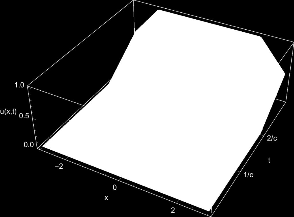
18 Example: Plucked String Determine the solution to the initial value problem: u tt = c 2 u xx for < x < and t > 0 { 2 if 1 < x < 1 u(x, 0) = f (x) = 0 otherwise u t (x, 0) = 0

19 Solution (1 of 7) Using d Alembert s solution u(x, t) = 1 [f (x + c t) + f (x c t)]. 2 Note: Along lines where x + c t is constant the term f (x + c t) is constant. Likewise along lines where x c t is constant the term f (x c t) is constant. These lines are called characteristics.

20 Solution (2 of 7) f (x) = f (x + c t) = 1 f (x + c t) = 2 { 2 if 1 < x < 1 0 otherwise { 2 if 1 < x + c t < 1 0 otherwise { 1 if 1 c t < x < 1 c t 0 otherwise

21 Solution (2 of 7) f (x) = f (x + c t) = 1 f (x + c t) = 2 1 f (x c t) = 2 { 2 if 1 < x < 1 0 otherwise { 2 if 1 < x + c t < 1 0 otherwise { 1 if 1 c t < x < 1 c t 0 otherwise { 1 if 1 + c t < x < 1 + c t 0 otherwise

22 Solution (2 of 7) f (x) = f (x + c t) = 1 f (x + c t) = 2 1 f (x c t) = 2 { 2 if 1 < x < 1 0 otherwise { 2 if 1 < x + c t < 1 0 otherwise { 1 if 1 c t < x < 1 c t 0 otherwise { 1 if 1 + c t < x < 1 + c t 0 otherwise Remark: the characteristics where x + c t = ±1 and x c t = ±1 help determine the solution.

23 t Solution (3 of 7) Region 6 Region 5 Region 4 2/c 1/c Region 1 Region 2 Region 3 x - c t = -1 x - c t = 1 x + c t = -1 x + c t = x

24 Solution (4 of 7) Region 1: {(x, t) x + c t < 1} Region 2: {(x, t) 1 < x c t and x + c t < 1} Region 3: {(x, t) 1 < x c t} Region 4: {(x, t) 1 < x + c t and 1 < x c t < 1} Region 5: {(x, t) 1 < x + c t and x c t < 1} Region 6: {(x, t) 1 < x + c t < 1 and x c t < 1}

25 Solution (5 of 7) u(x, t) = 1 2 f (x + c t) + 1 f (x c t) 2 0 if x + c t < 1 2 if 1 < x c t < 1 and 1 < x + c t < 1 0 if 1 < x c t = 1 if 1 < x + c t and 1 < x c t < 1 0 if 1 < x + c t and x c t < 1 1 if 1 < x + c t < 1 and x c t < 1

26 t Solution (6 of 7) 2/c 1/c u=0 u=1 u=1 u=0 u=2 u= x x - c t = -1 x - c t = 1 x + c t = -1 x + c t = 1

27 Solution (7 of 7)

28 Example: Struck String Determine the solution to the initial value problem: u tt = c 2 u xx for < x < and t > 0 u(x, 0) = 0 u t (x, 0) = g(x) = { 1 if 1 < x < 1 0 otherwise

29 Solution (1 of 6) Define the function G(z) = z 0 1 if z < 1 g(w) dw = z if 1 z 1 1 if z > 1. then u(x, t) = 1 [G(x + c t) G(x c t)]. 2c As in the previous example, the characteristics x + c t = ±1 and x c t = ±1 divide the xt-plane into six regions.

30 t Solution (2 of 6) Region 6 Region 5 Region 4 2/c 1/c Region 1 Region 2 Region 3 x - c t = -1 x - c t = 1 x + c t = -1 x + c t = x

31 Solution (3 of 6) Region 1: {(x, t) x + c t < 1} Region 2: {(x, t) 1 < x c t and x + c t < 1} Region 3: {(x, t) 1 < x c t} Region 4: {(x, t) 1 < x + c t and 1 < x c t < 1} Region 5: {(x, t) 1 < x + c t and x c t < 1} Region 6: {(x, t) 1 < x + c t < 1 and x c t < 1}

32 Solution (4 of 6) u(x, t) = 1 2c G(x + c t) 1 G(x c t) 2c 0 if x + c t < 1 2c t if 1 < x c t and x + c t < 1 = 1 0 if 1 < x c t 2c 1 x + c t if 1 < x + c t and 1 < x c t < 1 2 if 1 < x + c t and x c t < x + c t if x c t < 1 and 1 < x + c t < 1

33 Solution (5 of 6) 2/c x - c t = -1 t x-ct=1 x + c t = -1 1/c x+ct= x 1 2 3

34 Solution (6 of 6)

35 Domain of Dependence (1 of 2) In general the solution to the initial value problem: u tt = c 2 u xx for < x < and t > 0 u(x, 0) = f (x) u t (x, 0) = g(x) can be expressed as u(x, t) = 1 2 [f (x + c t) + f (x c t)] + 1 2c At the point (x 0, t 0 ) then u(x 0, t 0 ) = 1 2 [f (x 0 + c t 0 ) + f (x 0 c t 0 )] + 1 2c x+c t x c t x0 +c t 0 x 0 c t 0 g(s) ds. g(s) ds.

36 Domain of Dependence (2 of 2) u(x 0, t 0 ) = 1 2 [f (x 0 + c t 0 ) + f (x 0 c t 0 )] + 1 2c x0 +c t 0 x 0 c t 0 g(s) ds. Remarks: u(x 0, t 0 ) depends only on the values of f (x 0 ± c t) and g(s) for x 0 c t 0 s x 0 + c t 0. The interval [x 0 c t 0, x 0 + c t 0 ] is called the domain of dependence.

37 Domain of Dependence Illustrated t 0 t (x 0, t 0 ) x 0 - c t 0 x 0 x 0 + c t 0 x

38 Domain of Influence The point (x 0, t 0 ) influences the solution u(x, t) for t t 0 at all points between the characteristics passing through (x 0, t 0 ). t t 0 = ±1 x x 0 c c(t t 0 ) = ±(x x 0 ) ±x 0 + c(t t 0 ) = ±x

39 Domain of Influence Illustrated t x = x 0 - c(t - t 0 ) x = x 0 + c(t - t 0 ) t 0 (x 0, t 0 ) x 0 x

40 Finite Length String D Alembert s solution to the wave equation can be adapted to the wave equation with 0 < x < L. u tt = c 2 u xx for 0 < x < L and t > 0 u(0, t) = u(l, t) = 0 u(x, 0) = f (x) u t (x, 0) = g(x)

41 Case: Plucked String u tt = c 2 u xx for 0 < x < L and t > 0 u(0, t) = u(l, t) = 0 u(x, 0) = f (x) u t (x, 0) = 0 We have used separation of variables and Fourier series to determine u(x, t) = a n cos c n π t sin n π x L L n=1

42 Case: Plucked String u tt = c 2 u xx for 0 < x < L and t > 0 u(0, t) = u(l, t) = 0 u(x, 0) = f (x) u t (x, 0) = 0 We have used separation of variables and Fourier series to determine u(x, t) = a n cos c n π t sin n π x L L n=1 [ = 1 ] nπ(x + c t) nπ(x c t) a n sin + a n sin 2 L L n=1 n=1 = 1 [f (x + c t) + f (x c t)], 2 where f (x) is the odd, 2L-periodic extension of the initial displacement.

43 Case: Struck String u tt = c 2 u xx for 0 < x < L and t > 0 u(0, t) = u(l, t) = 0 u(l, t) = 0 u(x, 0) = 0 u t (x, 0) = g(x) We have used separation of variables and Fourier series to determine u(x, t) = n=1 b n sin c n π t L sin n π x L

44 Case: Struck String u tt = c 2 u xx for 0 < x < L and t > 0 u(0, t) = u(l, t) = 0 u(l, t) = 0 u(x, 0) = 0 u t (x, 0) = g(x) We have used separation of variables and Fourier series to determine u(x, t) = = 1 2 b n sin c n π t L n=1 n=1 sin n π x L [ nπ(x c t) b n cos b n cos L ] nπ(x + c t). L

45 Integrating Term by Term u(x, t) = 1 2 = 1 2 = 1 2 = 1 2c = 1 2c [ nπ(x c t) b n cos b n cos L n=1 nπ x+c t b n sin nπs L x c t L ds ( ) [ nπ ] b n sin nπs ds L L n=1 x+c t x c t n=1 x+c t x c t x+c t x c t ( [ n=1 g(s) ds b n cnπ L ] sin nπs L ) ] nπ(x + c t) L where g(x) is the odd, 2L-periodic extension of the initial velocity. ds

46 Example Find the solution to the initial boundary value problem u tt = 4u xx for 0 < x < 1 and t > 0 u(0, t) = u(l, t) = 0 u(x, 0) = 0 u t (x, 0) = 0 if x < 1/4 1 if 1/4 x 3/4 0 if 3/4 < x < 1. Let g(x) be the odd, 2-periodic extension of u t (x, 0).

47 Solution (1 of 6) Let g o (x) be the odd, 2-periodic extension of u t (x, 0). g o (x) = 0 if 0 < x < 1/4 1 if 1/4 < x < 3/4 0 if 3/4 < x < 5/4 1 if 5/4 < x < 7/4 0 if 7/4 < x < 2

48 Solution (2 of 6) g o (x) x

49 Solution (3 of 6) Define the function G(x) = x 0 g o (s) ds.

50 Solution (3 of 6) Define the function G(x) = G(x) = = x 0 g o (s) ds. x 0 0 ds if x < 1/4 x 1/4 1 ds if 1/4 x 3/4 3/4 1/4 1 ds if 3/4 < x < 5/4 1/4 1 ds + x 5/4 ( 1) ds if 5/4 < x < 7/4 1/4 1 ds + 7/4 5/4 ( 1) ds if 7/4 < x < 2 3/4 3/4 0 if x < 1/4 x 1/4 if 1/4 x 3/4 1/2 if 3/4 < x < 5/4 x + 7/4 if 5/4 < x < 7/4 0 if 7/4 < x < 2

51 Solution (4 of 6) G(x + 2t) = G(x 2t) = 0 if x + 2t < 1/4 x + 2t 1/4 if 1/4 x + 2t 3/4 1/2 if 3/4 < x + 2t < 5/4 x 2t + 7/4 if 5/4 < x + 2t < 7/4 0 if 7/4 < x + 2t < 2 0 if x 2t < 1/4 x 2t 1/4 if 1/4 x 2t 3/4 1/2 if 3/4 < x 2t < 5/4 x + 2t + 7/4 if 5/4 < x 2t < 7/4 0 if 7/4 < x 2t < 2

52 Solution (5 of 6) Using d Alembert s solution to the wave equation, then u(x, t) = 1 [G((x + c t) 2c (mod 2)) G((x c t) (mod 2))] = 1 [G((x + 2t) 4 (mod 2)) G((x 2t) (mod 2))].

53 Solution (6 of 6)

54 Homework Read Sections 5.2 and 5.3 Exercises: 6 10