Study of Water Cerenkov and Prototype Detector of Daya Bay Experiment
|
|
|
- Νίκη Μιχαλολιάκος
- 7 χρόνια πριν
- Προβολές:
Transcript
1 U D C : : : : : : : :
2 ii

3 Study of Water Cerenkov and Prototype Detector of Daya Bay Experiment Lu Haoqi In Partial Fulfillment of the Requirements for the Degree of Doctor of Philosophy Graduate School of Chinese Academy of Sciences Beijing, China 2009 ( Submitted in May 2009 )
4 iv c 2009 Lu Haoqi All Rights Reserved
5
6 vi
7 θ 13 θ 13 θ 13 sin 2 (2θ 13 ) 0.01 µ > 99.5%, 99.9%, PMT >30 tyvek > 80% µ tyvek 99% 140 ; µ ; :,,, tyvek,,,,
8 ii
9 Abstract Neutrino physics is the frontier of particle physics, astrophysics and cosmology. The neutrino mixing angle θ 13 is one of the fundamental parameters of the neutrino physics. The magnitude of θ 13 will decide the future direction of the neutrino physics. The Daya Bay neutrino experiment is proposed to measure the parameter θ 13 precisely using the reactor power plant group at Daya Bay, which is located in Shenzhen, Guangdong Province. To reach the sensitivity of 0.01 for sin 2 (2θ 13 ) measurement, one has to study the backgrounds of the experiment in details, to optimize the design of the detector, to manufacture the prototype of the detector, and to test its performance. This thesis is mainly work on the water Cerenkov detector and tank prototype experiment. The Daya Bay experiment is a low background experiment.the veto systems with effective efficiency > 99.5%, play very important role. This thesis is worked on the design and optimization the water Cerenkov veto detector. The final design is a octagonal water Cerenkov detector with double layer structure which effective efficiency can reach 99.9%. The criterion for the detector is the water absorption length should >30 meters and the tyvek reflectivity should > 80% from the simulation results. To do the detector study, we design and construct prototype tank based on the Daya Bay pool. Based on the detector study, we construct a practical model try to estimate the water resistivity of the pool in final, which can be used for large water Cerenkov detector. The prototype measurement shows that the tyvek reflectivity can reach 99% and water absorption length can achieve 140m from the cosmic muon waveform study. It verifies that the Daya Bay experiment s criterion is practical. From the consistence between the cosmic muon data and MC results, the reliability and effectiveness of the water Cerenkov detector simulation software is verified. The construction and test of the tank prototype can provide the technique and experience for the construction of Daya Bay water Cerenkov detector. Key words: neutrino, Daya Bay reactor neutrino experiment, water Cerenkov detector, tyvek, efficiency, absorption length, reflectiviy,resistivity.
10 iv
11 sin 2 2θ v
12 vi Geant PMT Tyvek µ µ
13 vii Tyvek PMT µ µ µ RPC ( )
14 viii Tyvek µ µ µ µ µ
15 1 1.1 β 1914 β β (W. Pauli) 1930 β [1] [2] [3] [4] 1956 (F. Reines) (C. Cowan) [5] [6] [7] V-A [8] [9] 1958 [10] Glashow-Weinberg-Salam [11] SU(2) L U(1) Y SU(2) L Higgs [12] Yukawa [13] [14] τ [15] b [16] t [17] [18] Pontecorvo 1957 ν e ν e [19] 1962 Maki Nakagawa Sakata [20] ν e ν µ 1
16 2 1 Pontecorvo [21] Super-Kamiokande(SK) [22] K2K [23] MINOS [24] Homestake [25] 2002 SNO [26] ν e ν µ Mikheev-Smirnov-Wolfenstein(MSW) [27] [28] Kamland [29] SNO [30] 1.2 ν 1, ν 2, ν 3 ν e, ν µ, ν τ Maki-Nakagawa-Sakata-Pontecorvo (MNSP) [31] [32] ν α > = i U αi ν i > ( 1.1) α = e, µ, τ i = 1, 2, 3 ν i > Shrödinger ν i τ i m i ν i (τ i ) > = e im iτ i ν i (0) > ( 1.2) t L Lorentz e im iτ i = e i(e it P i L) ( 1.3) E i P i t L ν α P E i = p 2 + m 2 i P + m2 i 2P ( 1.4)
17 : ν i (τ i ) > e i m 2 i 2P L ν i (0) > ( 1.5) E P 1.6 ν α (L) > Uαi e im2 i L 2E U βi ν β > ( 1.6) β ı L < ν β ν α (L) > 2 L ν α ν β 1.7 [33] P(ν α ν β ) = δ αβ 4 i>j +2 i>j ( )] L Re(Uαi U βiu αj Uβj [1.27 )sin2 m 2 ij E ( )] L Im(Uαi U βiu αj Uβj [2.54 )sin m 2 ij E ( 1.7) m 2 ij m 2 i m2 j ev 2 L km E GeV 1.27 [34] CPT P( ν α ν β ) = P(ν β ν α ) ( 1.8) 1.7 P(ν β ν α, U) = P(ν α ν β, U ) ( 1.9) CPT 1.10 P( ν α ν β, U) = P(ν α ν β, U ) ( 1.10) U U 1.7 CPT CP [33] MNSP [35] [36] c 13 0 s 13 e iδ c 12 s 12 0 U = 0 c 23 s s 12 c s 23 c 23 s 13 e iδ 0 c
18 4 1 e iφ e iφ ( 1.11) = c 12 c 13 s 12 c 13 s 13 e iδ s 12 c 23 c 12 s 23 s 13 e iδ c 12 c 23 s 12 s 23 s 13 e iδ s 23 c 13 s 12 s 23 c 12 c 23 s 13 e iδ c 12 s 23 s 12 c 23 s 13 e iδ c 23 c 13 e iφ e iφ ( 1.12) s ij = sin θ ij, c ij = cosθ ij, (i, j = 1, 2, 3) φ 1, φ 2 φ 1, φ 2 Majorana Majorana β (neutrinoless double beta decay) 2. CP Jarlskog [37] U Jarlskog Jarlskog J CP = s 12 c 12 s 23 c 23 s 13 c 2 13 sin δ ( 1.13) CP sin δ 1.11 δ CP CP/T CP CP δ m 2 21 = m 2 solar, m 2 32 = m 2 atom, θ 12 = θ solar, θ 23 = θ atom,
19 θ 13 = θ reactor. ( 1.14) solar θ 12 m 2 21 (SNO ) (KamLAND) 5σ atom θ 23 m 2 32 (SuperK ) (MINOS) 5σ reactor θ 13 KamLand SNO [38] [39] m 2 21 = ev 2, sin 2 (2θ 12 ) = ( 1.15) K2K Super-K [38] [40] m 2 32 = ( ) 10 3 ev 2, sin 2 (2θ 23 ) > 0.92 (90% Confidence Level) ( 1.16) CHOOZ Palo Verde [38] [41] sin 2 (2θ 13 ) < 0.13 (90% Confidence Level) ( 1.17) 1.18 m m m2 13 = 0 ( 1.18) m 2 12, m2 32, sin2 (θ 12 ), sin 2 (θ 23 ), sin 2 (θ 13 ), δ ( 1.19) m 2 12, m2 32, sin2 (θ 12 ), sin 2 (θ 23 ) sign of m 2 32, sin 2 (θ 13 ), δ ( 1.20)
20 m 2 12 m ( 1.21) m 2 32 m 2 31 ( 1.22) 1.7 L/E m 2 L E = o(1) ( 1.23) 1.11 MNSP 1.7 P(ν α ν β ) = sin 2 2θ sin 2 [1.27 m 2 L/E] ( 1.24) β α P(ν α ν α ) = 1 sin 2 2θ sin 2 [1.27 m 2 L/E] ( 1.25) 1.24 (appearance) 1.25 (disappearance) MeV ν e 1.1 [42 45] ν e β 1.2 [46] 3 7MeV [47, 48] Kamioka [49] IMB [50] SuperK [51]
 ( ) β ( ) µ µ 50% (E) (L) Kamioka SuperK m 2 32 (K2K,MINIOS) L K2K [52] 2007 MINIOS [53,54] [55] m 2 32 = 2.")
21 : 1.2: ( ) ( ) β ( ) µ µ 50% (E) (L) Kamioka SuperK m 2 32 (K2K,MINIOS) L K2K [52] 2007 MINIOS [53,54] [55] m 2 32 = ev 2, sin 2 θ 23 = ( 1.26) ν e, 1.1 Ray Davis Homestake ν e + Cl e + Ar [43] (SSM) Davis
22 GALLEX [45] SAGE [44] ν e +Ga e+ge SuperK ν e + e ν e + e ν e [56] MeV µ τ ν e ν e ν µ ν τ 2000 SNO ν e +d p+p+e ν+d ν+n+p [57] SNO ν e (1.68 ± 0.06(stat) (sys)) 10 6 cm 2 s 1 [58 60] (4.94 ± 0.21(stat) (sys)) 106 cm 2 s 1 [58 60] ν e ν µ ν τ KamLAND m 2 KamLAND 51 L/E 10 6 m/mev m 2 tan 2 θ 12 = m 2 21 = ev 2 MSW [55] m 2 21 = ev 2, ( 1.27) sin 2 θ 12 = ( 1.28) K2K,MINOS, Kamland θ 13 CHOOZ [61] CHOOZ 1km β ν e + p e + + n ( 1.29) θ CHOOZ sin 2 (2θ 13 ) θ 13 :sin 2 θ 13 < 0.036(2σ) [55]
23 1.4. sin 2 2θ : 90% m 2 sin 2 2θ CHOOZ Palo Verde Kamiokande [62] 1.1: 95% m 2 21 = ev 2 ( ) 10 5 ev 2 m 2 32 = ev 2 ( ) 10 3 ev 2 sin 2 θ 12= < sin 2 θ 12 < sin 2 θ 23= < sin 2 θ 23 < θ 13 sin 2 θ 13=0.016 sin 2 θ 13 < [55] 1.4 sin 2 2θ 13 CHOOZ sin 2 2θ 13 θ 13 < θ C 13 θ C Cabibbo θ 12 θ 23 θ 13 θ Jarlskog CP
24 10 1 sin 2 2θ 13 CP χ χ 2 vs θ 13 All [p-p] ν-e ± 1% χ sin 2 θ σ 90% CL Total Atm + K2K + Chooz sin 2 θ 13 Solar + KamLAND 10-1 KamLAND Solar 1.4: χ 2 sin 2 θ 13 BGP [64] MSTV [65] θ 13 [63] [64] [65] θ m 2 12 m 2 23 CP θ 12, θ 23, θ 13, m 2 21, m2 32 χ 2 sin 2 θ 13 = BGP sin 2 θ 13 = MSTV 1.2 2σ 3σ BGP MSTV θ 13 3σ θ C BGP MSTV θ sin 2 2θ 13 (2 3)% 1% θ 13 [35] % θ [66] sin 2 (2θ 13 ) = 0 ± 0.05 ( 1.30)
25 1.4. sin 2 2θ Parameter (BGP [64]) Best fit 2σ interval 3σ interval m 2 21 (10 5 ev 2 ) m 2 32 (10 3 ev 2 ) tan 2 θ tan 2 θ sin 2 θ 13 (sin 2 2θ 13 ) (0.036) Parameter (MSTV [65]) Best fit 2σ interval 3σ interval m 2 21 (10 5 ev 2 ) m 2 31 (10 3 ev 2 ) sin 2 θ sin 2 θ sin 2 θ 13 (sin 2 2θ 13 ) (0.024) : 2σ (95% C.L.) 3σ (99.7% C.L.) [35] θ 13 < 10 (99% Confidence Level) ( 1.31) % θ [55] θ 13 CHOOZ θ 13 ν µ ν e ν τ CP [38] P(ν µ ν τ ) = sin 2 2θ 23 cos 4 θ 13 sin 2 [1.27 m 2 32L/E] ( 1.32) P(ν µ ν e ) = sin 2 2θ 13 sin 2 θ 12 sin 2 [1.27 m 2 32L/E] ( 1.33) θ 13 ν µ ν τ ν µ ν e θ 13 CP P(ν µ ν e ) = sin 2 2θ 13 sin 2 θ 23 sin 2 [1.27 m 2 32L/E] + sin 2 2θ 13 cos 2 θ 23 sin 2 [1.27 m 2 21 L/E] (+)J sin(δ) sin[1.27 m 2 32 L/E] +J cos(δ) cos[1.27 m 2 32L/E] ( 1.34)
26 12 1 J Jarlskog [38] 1.34 θ 13 [67]: i δ, θ 13 ii m 2 32 iii θ 23, π θ 2 23 δ CP θ 13 [38] P( ν e ν e ) = 1 cos 4 θ 13 sin 2 2θ 12 sin 2 [1.27 m 2 21 L/E] sin 2 2θ 13 sin 2 [1.27 m 2 32L/E] ( 1.35) L < 5km θ 13 CP θ 13

27 2 2.1 θ GW 5.8GW : sin 2 2θ 13 90% sin 2 2θ [68] 13
 ( ) 2.2 2.2: 2. 3. µ µ 4. µ µ 99.")
28 sin 2 2θ CHOOZ sin 2 2θ 13 < 0.17 CHOOZ 1. ( ) ( ) : µ µ 4. µ µ 99.5% µ
 2.")
29 : χ 2 m 2.2 χ 2 ( 2.3) 2.3 (AD) µ RPC
30 Gd β 5m 5m ( ) I Gd0.1% 20 II (fiducial volume) III 192 ( PMT) 8 12% 2.4: 2.5:
31 ( 2.6) ν e + p e + + n ( 2.1) 2.6: β β 2.2MeV 8MeV 0.1% 28 Gd 210us) Gd 3-4 8MeV γ 3.5MeV µ γ µ 2.5m 1 2MeV γ 2.5m γ 6 ( 2.7 ) 2.8
 µ 2.9 2.")

32 : γ 2.8: (RPC) µ : 2.10: ( ) m
33 : µ 99.5% µ ±0.25% 25% ±0.05% 0.5-1m RPC ±2ns 25ns 2m m 2.5m Tyvek tyvek 0.8% 1m RPC 2m 2m 18m 18m 18m 12m RPC 1m 4 RPC RPC RPC RPC 95% 98.6%( ) RPC x y RPC µ (<10cm) RPC µ µ RPC RPC µ 99.5% 0.25% µ µ (>30 ) 2
34 : 363m 481m 1985m -II 526m 1615m (m) (Hz) < 50 < 50 < 50 µ (Hz) ( / ) (%) < 0.2 < 0.2 < 0.1 (%) He 9 Li (%) / 5 /10 5 / 10 / 8 / θ 13 θ 13 θ 13 θ 13 sin 2 (2θ 13 ) 0.01
35 :

36 : 90% sin 2 2θ 13 ( ) CHOOZ 2.5.2
37 µ
38 24 2
39 3 3.1 v = βc n (c/n) Cherenkov Radiation cosθ c (λ) = [c/n(λ)]/v, ( 3.1) θ c (λ) n(λ) λ v > c/n θ c Tamm Frank ze L L+dL λ λ+dλ dn d 2 N dλdl = 2παz2 sin 2 θ λ 2 c 1 λ2, ( 3.2) α (α 1/137) λ = c/v = hc/e
40 26 3 d 2 N dedl = 2παz2 sin 2 θ c = constant. ( 3.3) hc E E λ = 1240eV nm dn λ1 dl = 2παz2 sin 2 θ c (λ, L)( dλ λ1 λ 2 λ ) = 2 2παz2 (1 (1/β 2 n 2 ))( dλ ), ( 3.4) λ 2 λ2 λ 1 λ dn 370(1 1/(n 2 β 2 ))dpdx. ( 3.5) β = 1 300nm 600nm photons/cm β 1 0.3KeV/cm 400KeV/cm 4KeV/cm 2300KeV/cm GEANT4 [69,70] FORTRAN GEANT3 GEANT4 C Geant4 Geant4 Geant4 λ 10nm E 100eV [71] G4dyb [200, 800]nm Geant4
41 Geant4 θ c ( 3.1 ) (BoundaryProcess) Geant4 (ABSLENGTH) Geant4 (RayleighAttenuationLength) Geant4 Einstein-Smoluchowski Geant4 Geant4 [72] (RINDEX) Geant4 (Fresnel formula) (surface) Geant4 GLISUR UNIFIED GLIUSR GEANT3 (POLISHED) (GROUND) UNIFIED [73] DETECT [74] UNIFIED 3.1 d i d r d t n 1 n 2 n θ i θ r θ t
 (polishedbackpainted) (groundbackpainted) (polishedfrontpainted) (groundfrontpainted) 3.")
42 28 3 φ r n α φ norm θ i θ r θ t UNIFIED (Type) (dielectric-dielectric) / (dielectric-metal) (Finish) (polished) (ground) (polishedbackpainted) (groundbackpainted) (polishedfrontpainted) (groundfrontpainted) 3.1: UNIFIED ( UNIFIED UNIFIED )
43 UNIFIED 3.1 J U (θ i, θ r, φ r ) R(θ i, n 1, n 2 )[C sl g(α r ; 0, σ α ) + C ss δ(θ i θ r )δ(φ r ) + C bs δ(θ i + θ r )δ(φ r ) +C dl cos(θ r )] + T(θ t, n 1, n 2 )g(α t ; 0, σ α ) ( 3.6) g(α r ; 0, σ α ) 0 σ α α [0, 90 ] σ α 3.6 UNIFIED σ α R(REFLECTIVITY) R C sl (SPECULARLOBECONSTANT) C ss (SPECULARSPIKE- CONSTANT) C bs (BACKSCATTERCONSTANT) [75] C dl Lambertian (DIFFUSELOBECONSTANT) C sl + C ss + C bs + C dl = 1 ( 3.7) T = 1 R J U n 1 = n 2 T = 1 UNIFIED C sl = 1 σ α = 0 (polished) C sl = 1 σ α PMT Geant4 (sensitive detector) (hit) 8 PMT G4dyb PMT PMT GLG4sim PMT [76] G4dyb PMT PMT 8 PMT PMT PMT PMT
 Luxlevel0 PMT PMT PMT (A(θ,λ)) (R(θ,λ)) (T(θ,λ)) A(θ, λ) + R(θ, λ) + T(θ, λ) = 1 ( 3.")
44 30 3 PMT ( 3.2 ) PMT 3.2: PMT ( G4dyb 8 EMI PMT PMT Luxlevel3 ) 26nm i PMT (sensitive detector) Luxlevel0 PMT PMT PMT (A(θ,λ)) (R(θ,λ)) (T(θ,λ)) A(θ, λ) + R(θ, λ) + T(θ, λ) = 1 ( 3.8) PMT PMT PMT PMT PMT Luxlevel3 Luxlevel3 luxlevel0 50/50 PMT Luxlevel3 luxlevel0 Luxlevel3 Luxlevel0 [76]
45 : (g/cm 3 ) (g/cm 3 ) 1.0 H,O 2.7 O, Si, Al,Fe, Mg, K, Ca Gd C, H,N, O, Gd %Al, Si, Mn C, H,N, O ESR 1.0 C, H C, H Tyvek 0.94 C, H 1.18 C, H,O PMT 2.23 Si, O, B, Na %Fe, C, Mn PMT 5 K 3.2: (m) Tyvek 10 0 PMT PMT i G4dyb Parlo Verde Geant3 KamLAND GLG4sim G4dyb 3.2 Tyvek Tyvek Tyvek Tyvek, tyvek Super K Kamland Auger
46 : -tyvek UNIFIED -tyvek UNIFIED - UNIFIED tyvek, D tyvek 320nm 90% tyvek PMT [300nm-600nm]( 3.2 ) Tvyek Auger % Kamland tyvek 80% tyvek 0.1 tyvek 80% 90% 80% ( ) Diffuse reflectivity(%) wave length(nm) 3.3: Tyvek Geant4 ( ( ) 1 (n 2 1)(n 2 2 ( ) ) ) 2πp L Rayleigh = ktk T, ( 3.9) 6π 3 hc
47 h c p n k T K T Geant4 T = K K T = m 3 /MeV ( 3.4) SuperK 3.4: Gean4 [77] 3.5 [78 87] 350nm 600nm Pope Fry Quickenden Irvin Quickenden Irvin
48 34 3 Absorption coefficient (1/cm) Sogandares and Fry, 1997 Pope and Fry, 1997 Querry et al, 1991 Quickenden and Irvin, 1980 Tam and Patel, 1979 Querry, Cary and Waring, 1978 Kopelevich, 1976 Palmer and Williams, 1974 Sullivan, 1963 Quickenden and Irvin, Purity 1 Quickenden and Irvin, Purity Wavelength (nm) 3.5: [78 87] 200nm 800nm a min (200nm-320nm) Quickenden Irvin1980, (380nm-727.5nm) Pope Fry ( nm) Sullivan Sullivan 800nm (10% ) [82] 25 [80] 22 a i = a i(200nm) (λ/200nm) 4 a i (200nm) 200nm 1/λ 4 Rayleigh 3.6 a = a min + a i a i (200nm) = 0 ( ) 226m 417nm 3.7 a i (200nm) Rayleigh
49 Absorption coefficient (1/cm) Sogandares and Fry, 1997 Pope and Fry, 1997 Querry et al, 1991 Quickenden and Irvin, 1980 Tam and Patel, 1979 Querry, Cary and Waring, 1978 Kopelevich, 1976 Palmer and Williams, 1974 Sullivan, 1963 Quickenden and Irvin, Purity 1 Quickenden and Irvin, Purity 2 Fake (30.0m, 473nm) Fake (53.4m, 435nm) Fake (226m, 417nm) Wavelength (nm) 3.6: 3.7: G4dyb [88, 89] 1 PVC tyvek WinstonCone [90] EMI 8 PMT tyvek Winston Cone µ, : [88]
50 tyvek (90%) Al ( 90%) PMT PMT µ PMT e x/λ x µ PMT λ tyvek µ PMT 5.7± : tyvek,al PMT [88] 3.10: µ 5.7 ± 0.3m [88] G4dyb 3.11 G4dyb 3.3 >95% µ >99.5% <0.25%
51 number of detected photons 10 Exp.data MC distance/m 3.11: G4dyb µ [91] µ µ (Gaisser s formula) MUSIC( µ ) µ µ 3.4 µ µ (m) µ (Hz/m 2 ) (GeV) : µ
52 38 3 /GeV ) 2 muon flux ( Hz/m far midle DaYa near LingAo near site underground muon energy ( GeV ) counts far midle DaYa near LingAo near site cos(θ) of underground muon 3.12: µ : µ 3.12 ( ) µ µ 3.13 µ 75 µ MUSIC µ θ > 75 µ θ > 75 µ µ µ 3.14 x z counts far midle DaYa near LingAo near site azimuthal angle of underground muon 3.14: µ 250 µ
53 µ µ 200 1% PMT 50Hz PMT PMT PMT PMT N n ( PMT ) f τ R = 1 τ N icn(fτ) i i (1 fτ) N i ; ( 3.10) i=n 3.15: PMT ( PMT 200 PMT 50kHz 100ns) PMT PMT PMT 3.15 PMT PMT PMT MACRO PMT( 400 ) PMT PMT <5kHz MACRO PMT PMT
54 kHz PMT <5kHz PMT 50kHz 50kHz 3.16 ( tyvek 80% max. 20m) Hittimedis Entries Mean RMS 30 collect p.e. ratio (%) photon hit time(ns) 3.16: time window (ns) 3.17: ns 99.8% 200ns E effi = n detect N Inwater ( 3.11) n detect µ N Inwater µ µ µ PMT tyvek PMT µ
55 m*14m*9m 1.5m 3.18: (4 ( ) PMT) PMT 1.52 PMT PMT 321 tyvek 0.8( tyvek ) 20 ( ) µ 5.5m 4m 9m 400 htracklengthinner Entries Mean RMS Tracklength in water(m) 3.19: µ 3.20 PMT 25ns 200ns (99% ) 3.21 µ
56 42 3 PMTs µ 3.22 PMT µ PMT PMT 100 µ 100 PMT Hittimedis Entries Mean RMS p.e. hit time(ns) 3.20: PMT Hittimedis Entries Mean RMS Output p.e. number 3.21: PMT Hittimedis Entries Mean RMS p.e number per PMT for all muons 3.22: PMT Hittimedis Entries Mean 100 RMS Fired PMT number 3.23: PMT

57 : 3.25: PVC PVC 3.26 PVC PVC 1m % 70%
58 m 70% µ 3.26: PVC 3.27: [88] m 1m PVC tyvek 1m 16m*1m*1m PVC 16 9 PMT µ 3.29 Winstone Cone Winstone
(c) 45 PMT 3.31 16 3.10 µ PMT10.5 PMT 7 16 µ PMT 7.0 e 16.0 10.5 5.7 2.")
59 : 1m 1m µ µ Windstone 3.29 (b) PMT ( 3.29(b) ) (b) ( ) (c) 45 PMT ( 16m 16m 10m ) (a) 16m 1m 1m (b)(c) 45 PMT µ PMT10.5 PMT 7 16 µ PMT 7.0 e ( tyvek 90%, 30 ) PMT PMT PMT µ PMT PMTs PMT 8 PMT PMT 416
60 : 3.30: 3.32 µ 100 ( 3.21)
 µ ( ) tyvek PMT A B 3.36 3.")
61 : PMT µ µ 2 3 PMT 3.34 PMT h1 Entries 1000 Mean RMS Output p.e. number : h1 Entries 1000 Mean RMS Fired PMT number 3.33: PMT 3.35 µ ( ) µ ( ) tyvek PMT A B µ X 7
 A 0.88 89 B 491 4 B 1 A 15 A B A PMTs µ 3.35: µ 3.38 µ A PMTs -7 +7 491 0.")
62 h1 Entries Mean RMS p.e number per PMT for all muons 3.34: PMT ( µ ) A B B 1 A 15 A B A PMTs µ 3.35: µ 3.38 µ A PMTs µ µ
63 h1 Entries 1000 Mean RMS h2 Entries 1000 Mean 491 RMS h1 Entries 568 Mean RMS h2 Entries 1000 Mean RMS PMTs output p.e. number at A PMTs output p.e. number at at B PMTs hit time at A (ns) PMTs hit time at B (ns) 3.36: µ (x=7 m) PMTs 3.37: µ (x=7 m) PMT p.e. number observed Distance (m) Hit time (ns) 90 χ 2 / ndf / p ± p ± Distance (m) 3.38: µ (x ) A PMTs ( 3.36 ) 3.39: µ (x ) A PMT ( 3.36 )
64 µ 2 3 µ PVC 16 PVC 16 µ µ tyvek PVC PVC PVC tyvek PMT µ PMT µ PMT PMT( ) µ (<1m) PMT 3.40 PMT ( 3.31) PMT 416 ( 3.40) PMT 1.5 PMT PMT PMT tyvek
65 : PMT PMT 1 PMT 200PMT µ PMT µ PMT 3.43 µ PMT 19 PMT 3.44 PMT PMT PMT µ µ µ µ µ <1m 3.45 µ 2 3 µ 3.36 µ (>5p.e.)

66 h1 Entries 1000 Mean RMS p.e number h1 Entries 1000 Mean 1752 RMS p.e number 3.41: 3.42: PMT h1 Entries 1000 Mean RMS h1 Entries 1000 Mean RMS fired PMT Number fired PMT Number 3.43: PMT 3.44: PMT PMT 3.45: µ 3.46: µ PMT
67 n = N exp( x/λ) n PMT λ 3.37 PMT µ X error = X re x 0 ; Y error = Y re y 0 ; Z error = Z re z 0 ; Re error = Xerror 2 + Y error 2 + Z2 error ; X Y re re, Z re x y z x y 0 z 0 0 µ Re error PMT µ PMT PMT µ PMT 4 6 PMT PMT X j re = n i=1 Npe i x j n i=1 Npe i ( 3.12) Xre j j=1 2 3 X Y Z x PMT Npe i PMT n PMT htemp Entries 827 Mean RMS htemp Entries 943 Mean RMS reconstruction_error 3.47:, reconstruction_error 3.48: PMT, PMT


68 PMT µ, htemp Entries 328 Mean RMS htemp Entries 368 Mean RMS reconstruction_error reconstruction_error 3.49:, 3.50: PMT, µ µ PMT 3.51 < ( PMT) 3.51: PMT 3.52: ( PMT)
69 : PMT PMT 341 PMT PMT 381 PMT PMT PMT (PMT 341) ( 381 PMT ) 341PMT PMT 3.56
70 : PMT 3.55: : µ 3.57: µ,
71 µ µ µ (<1.0 )µ (381 PMT) 96.1% 95.3% 97.1% 98.5% (341 PMT) 96.3% 97.0% 97.7% 98.9% (381 PMT) 96.5% 96.9% 97.9% 99.0% 3.5: 3.5 ( PMT 50kHz 200ns) 381 PMT, PMT p.e loss ICut Ieffi. OCut Oeffi. I or O effi. Total effi 50kHz 200 ns 0.1% % % 97.9% 99.0% 50kHz 150 ns 0.6% % % 98.2% 99.1% 50kHz 100 ns 3.2% % % 98.5% 98.2% 15kHz 200 ns 0.1% % % 98.9% 99.5% 15kHz 150 ns 0.6% % % 99.1% 99.6% 15kHz 100 ns 3.2% % % 99.1% 99.6% 3.6: (381PMT) PMT PMT PMT ( < ±0.2%) p.e. loss ICut PMT Ieffi. µ Oeffi. µ I or O effi. Total effi. RPC ( RPC 90%) 200ns 100ns 97.9% 98.5%( PMT 50kHz ) PMT 15kHz 98.9% 99.1%
72 ns 0.1% 100ns 3.2% µ 200ns 100ns 0.2% 200ns µ µ >99.5% µ µ E effective = 1 N undectnutron N gennutron ( 3.13) E effective N undectnutron µ µ N gennutron µ 3.57 µ 3.58 µ µ µ 2 3 µ ( ) µ ( ) µ [93] 3.60 µ ( ) λ=80.7; x N neutron = exp( x ) ( 3.14) λ 3.14, 3.61 [93] 45.2(
73 : µ 3.59: µ µ 3.60: µ 12.5cm bin) 3.62 µ bin 3.63 µ µ 3.64 µ µ 6 N neutron = 6.5 exp( x ) ( 3.15) λ
74 : : µ ( ) 3.63: µ 3.64: µ ( µ ) ( cm)
75 µ µ % µ 99.0% µ 99.9% 99.5% <0.1% 3.7 [94] 99.5% % (cm) Rate B/S Rate B/S % % % % 3.7: % µ % 3.8: [94] 15% 2.5m 1 15%

![5 [95] 3.](/docs-images/85/92243462/images/76-1.jpg "65 3.66 3.")


76 [95] : 3.66: 3.67: 3.68:
77 4 PMT 4.1 PMT PMT PMT µ µ µ µ 4 µ µ 9 µ 9 9 ( µ ) µ µ µ µ 63
78 : ( µ ) 400 innertracklength Entries Mean RMS muon tracklength in IWD/m outertracklength Entries Mean 2.53 RMS muon tracklength in OWD/m 4.2: µ ( ) µ ( ) PMT PMT tyvek tyvek 80% 20 40% PMT µ 5.5 ( ) ( 300nm 600nm PMT ) PMT 1.4% 0.8% 260
79 >400, 4.4 > PMT PMT IWDPE 400 Entries Mean RMS total number of p.e. for IWD IWDHitN 300 Entries Mean RMS number of phototubes hit 700 IWDPE Entries Mean RMS total number of p.e. for OWD IWDHitN Entries Mean RMS number of phototubes hit 4.3: PMT 4.4: PMT Tyvek tyvek 4.5 tyvek % 190% number of p.e. observed 600 inner water detector outer water detector Tyvek reflectivity/% number of phototubes hit 120 inner water detector outer water detector Tyvek reflectivity/% 4.5: tyvek 4.6 tyvek 0.8 tyvek % tyvek >0.8
80 66 4 muon efficiency/% inner water detector outer water detector Tyvek reflectivity/% 4.6: tyvek % PMT 64% 1.7% ( 4.8) ( ) PMT (>400) ( 95%) µ number of p.e. observed surface reflectivity/% number of phototubes hit surface reflectivity/% 4.7: Tyvek µ tyvek PMT
81 muon efficiency/% surface reflectivity/% 4.8: % PMT number of p.e. observed inner water detector 100 outer water detector water absorption length/m number of phototubes hit inner water detector outer water detector water absorption length/m 4.9: 4.10 µ 2 10 > % 2 10 > % >20 (>95%) >30m
82 68 4 muon efficiency/% inner water detector outer water detector water absorbtion length/m 4.10: PMT PMT (<5%) 5% PMT PMT % PMT PMT 97.1% 97.0% 0.3% 0.6% inner detector efficiency/% 4.11: ) outer detector efficiency/% 4.12: > 20m > 30m tyvek > 80%;
83 % PMT 0.6% 4.2 RPC µ µ µ µ µ RPC tyvek Super K Auger Kamland tyvek tyvek % 7% 0.6% % 15% 1.2% ( RPC) (30m) (97.94±0.17)% (98.07±0.15)% (98.61±0.13)% (99.30±0.09)% (15m) (96.41±0.22)% (91.13±0.3)% (97.47±0.16)% (98.66±0.12)% (10m) (94.18±0.27)% (83.11±0.38)% (96.11±0.20)% (98.13±0.14)% 4.1:
84 70 4 (30m)-(15m) (1.53±0.28)% (6.95±0.34)% (1.14±0.21)% (0.64±0.15)% (30m)-(10m) (3.76±0.32)% (14.96±0.41)% (2.5±0.24)% (1.17±0.17)% 4.2: µ µ µ µ PMT 15 <0.009Hz µ 12.8Hz > 10 3 <0.1% µ 1 µ 2 µ 3 µ 3 µ 4.14 µ ( 4.2 ) µ µ <1 < 1 µ <1 0 (1 2% 3 ) htracklength Entries 8598 Mean RMS TrackLength(m) 4.13: µ 4.14: µ ( ) µ
85 %, 3 µ ( µ ) 1 2% 3 µ 3 µ ( ) ( - ) 30m % (97.78±0.18)% (98.07±0.15)% (0.29±0.24)% 15m % (90.07±0.36)% (91.13±0.3)% (1.06±0.47)% 10m % (80.65±0.48)% (83.11±0.38)% (2.45±0.62)% 4.3: µ µ µ PMT 19 <0.04Hz > 10 3 <0.1% µ 1 µ 2 µ 3 µ 3 µ 4.15: µ 4.16 µ µ Y %, 3 µ 21%(
86 htracklength Entries 8032 Mean RMS htracklength Entries 6367 Mean RMS TrackLength(m) TrackLength(m) 4.16: ( ) 4.17: ( 0 ) ( ) ) V O = m 3 V i = 1850m 3 R = V i V O = 77.5% 22.5%, 21% 22.5%( ) 3 µ ( ) ( - ) 30m % (77.43±0.46)% (97.94±0.17)% (20.51±0.49)% 15m % 75.06±0.50)% (96.41±0.22)% (22.53±0.55) 10m % (73.74±0.54)% (94.18±0.27)% (20.44±0.60) 4.4: µ 4.20 µ µ >4.0 µ 100% µ ( 4.21) %

 4.20: AD µ ( ) 4.21: AD µ ( ) ( ) ( ) 30m 2078 100% (97.35±0.")
87 : AD µ 4.19: AD µ htracklength Entries 6855 Mean RMS htracklength Entries 8598 Mean RMS TrackLength(m) TrackLength(m) 4.20: AD µ ( ) 4.21: AD µ ( ) ( ) ( ) 30m % (97.35±0.35)% 15m % (83.88±0.78)% 10m % (70.07±0.96)% 4.5:
88 RPC RPC RPC RPC RPC RPC µ 1 µ ( RPC ) 2 3 µ RPC 50 µ RPC RPC 4 µ 5 µ 6 µ ( RPC ) 7 µ ( RPC ) 8 µ 9 µ RPC 1 µ µ RPC 1 µ 1 µ µ µ 1 µ 2 >0 <2 > µ µ 4 1 µ µ RPC µ 0, RPC, 1 µ 4 RPC, 4 1 µ 1%
 PMT 50PMT <2 PMT < 50 PMT >11 PMT >13 PMT <50 4.")
89 : µ 4.23: µ RPC 99% µ PMT 4.24: µ RPC 4.25 µ PMT µ PMT 2 2 ( ) PMT 50PMT <2 PMT < 50 PMT >11 PMT >13 PMT < PMT mu >0 RPC 98.9% (2,3,4
90 : µ PMT ( ) µ PMT µ )1.1% 4.27 µ, XY XZ 1 µ 1 µ RPC 2 µ ( ) RPC 3 4 µ ( ) 3 10 nhitrpc Entries 3125 Mean RMS nhit_rpc 4.26: PMT ( PMT >11 PMT >13 PMT <50) RPC 4 3 µ 4 RPC RPC
91 : µ XY µ XZ 4.28, RPC 4.29 RPC 1% 99% 1% RPC sys. efficiency(%)(3/4) True effi. - Check effi.(%) Check effi. True effi RPC efficiency(one layer)(%) RPC efficiency(one layer)(%) 4.28: RPC 4.29: µ
92 % 20% RPC 99% 1%
93 5 5.1 (>30m) tyvek (>80%) Super-Kamiokande ( >100m) tyvek 1 PMT ( 0.6%) tyvek tyvek µ PMT m 1.2m 1.3m( ) Tyvek tyvek tyvek tyvek 79
94 MACRO PMT 0.62% tyvek 1 1 PMT (0,0,0) Y X Z PMT (-30cm,0,- 50cm) PMT (-110cm,-50cm,-10cm) 5.3 µ PMT PMT PMT X tyvek PMT tyvek PMT µ PMT X -110 PMT PMT Y X 30 h 1 µ d d = h tan(θ) θ ( 1.33 θ =41.2 ) d=87.5 PMT d PMT L=160 X 57.5 PMT 5.1: 5.2: 5.4 [96] PVC
95 : : PMT µ (PP) (PE) (PVC) 4.25 (PVC) tyvek 5.5: 5.6 PMT ( 1cm) 5.7 PMT PMT


96 : PMT 5.6: PMT PMT 2 PMT PMT 5.8 tyvek tyvek tyvek 5 5.8: tyvek 5.9: tyvek

97 : , h
98 : 2 ( ) 2l/min 18l/min / <1l/min / 2% / (EC) (R) (σ=1/r), (TDS) TDS TDS (mg/l)=
99 : 0.5 EC (µs/cm) [97] 5.13 V tank u(1/h) (position 1) (position 2) σ tank 1 σ p 2 25 C 0.055uS/cm σ p 5.13: k( mg/(l*h)) ( t dt) d(0.5σ tank ) = 0.5(σ p σ tank )udt (V tank ) + kdt ( 5.1)
100 86 5 (EC)σ tank ( 5.1) σ tank = (σ p + 2kτ) + (σ 0 (σ p + 2kτ))exp( t τ ) ( 5.2) τ= V tank u ; σ 0 R tank R tank = 1 σ tank = ( 5.3) t, R tank 1 (σ p + 2kτ) + (σ 0 (σ p + 2kτ))exp( t τ ) ( 5.3) R tank = 1 (σ p + 2kτ) ( 5.4) 5.4 σ p k τ k ( mg/(l h)) ( 5.1) ( 5.5) ( 5.6) d(0.5σ tank ) = k dt ( 5.5) σ tank = σ 0 + 2k t ( 5.6) σ 0 ( 5.7): R tank = 1 σ tank = 1 σ 0 + 2k t ( 5.7) >18MΩ cm 4 PVC 150 PVC 2 PMT tyvek
101 l cm 2.0cm 150 <1MΩ cm 16.7MΩ cm( σ p =0.06µS/cm 16.7MΩ cm) ( ) 2 ( ) 3MΩ cm u 1 12 l/min 5.3 k τ σ k mg/(l h) τ= l/min l/min( u 2 ) 5.15 k mg/(l h) 12 l/min(u 1 ) τ= l/min 10.2MΩ cm 3.5MΩ cm 10.2MΩ cm k, σ 0
102 88 5 water resistivity/mω*cm χ 2 / ndf 25.4/23 k ± 3.4e-05 τ σ ± ± time/hour 5.14: ( u 1 12 l/min) water resistivity/mω*cm χ 2 / ndf 52.49/47 k ± 3.2e-05 τ σ ± ± time/hour 5.15: ( u 2 3 l/min) k mg/(l h) k k k PVC (PP) ( 0.5 m 2 ) ( 5.4) k τ 5 6 τ
103 water resistivity/mω*cm 14 χ 2 / ndf 19.83/ k σ ± 3.1e ± time/hour 5.16: ( u 2 12 l/min) water resistivity/mω*cm χ 2 / ndf 20.94/21 k σ ± 4.8e ± time/hour 5.17: ( u 2 3 l/min) tyvek 2
104 90 5 tyvek PMT : ( ) 5.18 tyvek V 1 V 2 u 1i u 2i u 1o u 2o u c u u 1i +u 2i =u ; u 1o +u 2o =u; u c =u 1i -u 1o τ 1 = V 1 u 1o ; σ 1 V 1 k 1 V 1 V 1 ( t dt) V 1 : ( 5.8), ( 5.9) d(0.5σ 1 ) = 0.5(σ mb σ 1 )u 1i dt V 1 + k 1 dt ( 5.8) σ 1 = (σ mb + 2k 1 τ) + c 01 exp( t τ 1 ) ( 5.9)
105 σ mb =0.06 µs/cm ;τ 1 = V 1 u 1i V 1 ;c 01 V 2, σ 02 V 2 k 2 ( t dt) d(0.5σ 2 ) = 0.5(σ mbu 2i + σ 1 u c u 20 σ 2 ) V 2 dt + k 2 dt ( 5.10) dσ 2 dt = (σ mbu 2i + σ 1 u c u 20 σ 2 ) V 2 + 2k 2 ( 5.11) dσ 2 dt = σ mbu 2i + ((σ mb + 2k 1 τ) + c 01exp( t τ 1 ))u c u 20 σ 2 + 2k 2 ( 5.12) V 2 A = σ mb + 2k 1 τ 1 ; a = u cc 01 V 2 ; b = σ mbu 2i + 2k 2 V 2 + u c A V 2 ; τ 2 = V 2 u 2o ; ( 5.13) dσ 2 dt = b σ 2τ 2 + a exp( t τ 1 ); ( 5.14) ( 5.24) σ 2 σ 2 = bτ 2(τ 1 τ 2 ) + aτ 1 τ 2 exp( t τ 1 ) + c 02 exp( t ) ( 5.15) τ 1 τ 2 τ 2 σ ( u l/h): σ = u 1oσ 1 + u 2o σ 2 u 1o + u 2o ; ( 5.16) : R = 1 σ = u u 1o σ 1 + u 2o σ 2 ; ( 5.17) V 1, σ mb = σ 1 ; 5.18 d(0.5σ 1 ) = 0.5(σ mb σ 1 )u 1i dt V 1 + k 1 dt ( 5.18) d(0.5σ 1 ) = k 1 dt; ( 5.19) σ 1 = 2k 1 t + c 01 ; ( 5.20)
106 92 5 V 2 σ 2 = σ mb ; d(0.5σ 2 ) = 0.5u c(σ 1 σ 2 ) V 2 dt + k 2 dt ( 5.21) dσ 2 dt = u cc k 2 V 2 V 2 a 1 = u cc k 2 V 2 V 2 + 2k 1u c t u c σ 2 ; ( 5.22) V 2 V 2 ; a 2 = 2k 1u c ; a 3 = u c ; ( 5.23) V 2 V 2 dσ 2 dt = a 1 + a 2 t a 3 σ 2 ; ( 5.24) ( 5.24) σ 2 σ 2 = a 1a 3 a 2 a a 2 a 3 t + c 02 exp( a 3 t); ( 5.25) : σ = u 1oσ 1 + u 2o σ 2 u 1o + u 2o ; ( 5.26) R = 1 σ = u u 1o σ 1 + u 2o σ 2 ; ( 5.27) tyvek ( 5.8) 5.19 tyvek 23 PMT (PMT 20cm) ( 5.20 ) 23 PMT 5.20 (a) (b) PMT tyvek tyvek tyvek 1 tyvek PE tyvek ( 5.21 )


107 : tyvek 5.20: (a) ;(b) tyvek : tyvek 5.22: tyvek 10 PMT tyvek (??) l/min

 k 2 =2.")
108 tyvek 1 MΩ cm 11 l/min 5.23: 5.24: Tyvek tyvek V 1 =2600 l V 2 =1400 l u= 11.5 l/min 5.25 u 1i u 1o k 1 k 2 c 01 c l/min; u 1i =10.3 l/min u 2i =1.2 l/min;u 1o =9.8 l/mi u 2o = 1.7 l/min u c =0.5 l/min u c 0 k 1 k 2 k 1 = mg/(l h) k 2 = mg/(l h) 12MΩ cm
109 : ( ) 5.26: 0.8 u=11.5 l/min 1MΩ cm 8MΩ cm ( 5.27) 4MΩ cm
110 MΩ cm tyvek 5.27: 5.28: 5.5 k k
111 PP P v mg/(m 2 h) k k = P v S V ( 5.28) (a) tyvek (b) (c) k a = k PP + k PMTbulb + k cirsys ; ( 5.29) k b = k a + (k steel + k tyvek ); ( 5.30) k c = k b + k FCC ; ( 5.31) k a k PP k PMTbulb PMT k cirsys ( ) k b (a) tyvek k steel k tyvek tyvek ; k c k b (k FCC ) 5.1: S/V m 2 m 3 Substance S(m 2 ) S/V PP( ) PE(tyvek ) SS( ) PMT FCC( ) x PP PE PMT 0.138x 0.287x 0.076x P FCC k a = S PP 0.138x V tank + S PMTbulb 0.076x V tank + k cirsys ; ( 5.32)
112 98 5 k b = k a + ( S steel x V tank + S tyvek 0.287x V tank ); ( 5.33) ( 5.33)-( 5.32) k c = k b + S FCC P FCC V tank ; ( 5.34) k b k a = ( S steel x V tank + S tyvek 0.287x V tank ); ( 5.35) k c k b = S FCC C FCC V tank ; ( 5.36) : k a = mg/(l h); k b1 = mg/(l h); k b2 = mg/(l h); k b = k b1 V 1 +k b2 V 2 V 1 +V 2 = = mg/(l h); k c1 = mg/(l h); k c2 = mg/(l h); k c = k c1 V 1 +k c2 V 2 V 1 +V 2 = mg/(l h); x = P SS = 30ng/(cm 2 h); ( 5.37) P PP = 4.1ng/(cm 2 h); ( 5.38) P FCC = 935ng/(cm 2 h) = 31 P SS ; ( 5.39) PE
113 : Material pollution value 1.0 (PVC) 4.25 (PVC) ( ) PMT PMT PE PMT 5.3: m 1 [98] S/V ( ) S/V ( ) PMT PMT PMT PMT PMT (config.a config.b) 5.4 k mg/(l h), mg/(l h) 5.29 (
114 : S/V m 1 S/V ( ) (config.a) (config.b) (PE) PMT PMT PMT 0.03 k(10 3 mg/(l h)) : 5.40) R tank = 1 σ tank = 1 (σ p + 2kτ) + (σ 0 (σ p + 2kτ))exp( t τ ) ( 5.40) k τ k τ τ=1232./5.=246.4 ( 10 ) 5MΩ cm 1MΩ cm MΩ cm 4.1MΩ cm
115 5.6. µ water resistivity/mω*cm config.a config.a config.b config.b σ 0 =1 MΩ*cm σ 0 =5 MΩ*cm σ 0 =1 MΩ*cm σ 0 =5 MΩ*cm time/day : 5.5: S/V m 1 S/V ( ) (config.a) (config.b) 0.12 (PE) PMT PMT PMT k(10 3 mg/(l h)) k τ=1995.6/8.=249.4 ( 10 ) MΩ cm 4.5MΩ cm 5.6 µ µ µ tyvek
116 water resistivity/mω*cm config.a config.a config.b config.b σ 0 =1 MΩ*cm σ 0 =5 MΩ*cm σ 0 =1 MΩ*cm σ 0 =5 MΩ*cm time/day : µ µ µ 5.32 µ µ tyvek PMT PMT MOhms*cm 5.32: µ 1 µ 5.33 µ PMT
117 5.6. µ 103 1GHz 1ns 2us 5.34 µ 400ns tyvek tyvek tyvek PMT i(t) ; i(t) = 1 τ 0 e t τ 0 ( 5.41) PMT g(t): g(t) = 1 2πσ e (t t 0 )2 2σ 2 ( 5.42) t 0 PMT RC e t/rc PMT I(t) = i(t) g(t) 1 RC e t/rc ( 5.43) PMT 5.33: µ I(t) PMT µ µ PMT PMT I(t) τ 0 PMT
 c 5.35: PMT 5.")
118 : µ τ 0 =142ns τ 0 =138ns 140ns 5ns τ 0 =(140±5)ns L= n water tau 0 =0.3/1.33*140 m= 31.6 m [88] 5.7 ( tyvek 92%, 30 ) c 5.35: PMT 5.36: PMT 2) µ µ tyvek PMT µ µ PMT µ PMT 5.37 PMT
119 5.6. µ 105 ADC 400ns ADC 2249W, 2048, 5.38 µ PMT µ 1 tyvek 1 1 ADC 0.25 ADC PMT PMT PMT 5.37: µ histo0 Entries Mean 1250 RMS ADC channel 5.38: µ ADC a) PMT
120 NIM [99] ( ) n P(n, µ) = µn e µ n! ( 5.44) µ = mq m q µ n G n (x, Q 1, σ 1 ) = 1 e (x nq 1 ) 2 2nσ 1 2 ( 5.45) σ 1 2πn Q 1 σ 1 x n 0 δ S ideal (x, µ, Q 1, σ 1 ) = P(n, µ) G n (x, Q 1, σ 1 ) ( 5.46) 5.47 B(x, w, σ 0, α) = 1 w e x 2 2σ wθ(x)α e αx ( 5.47) σ 0 2π θ(x) θ(x) = { 0 x<0 1 x 0 ( 5.48)
121 5.6. µ 107 w σ 0 α S real (x) = S ideal (x, µ, Q 1, σ 1 ) B(x, w, σ 0, α) ( 5.49) Nr. of events χ 2 / ndf / 40 mu ± ped 12.1 ± 0.0 pdelta ± ph.e ± pedelta ± w ± A ± ADC channel 5.39: LED ph.e. Counts penumber Entries 1929 Mean RMS Number of photoelectron 5.40: PMT PMT PMT ( ) LED PMT LED PMT p.e.= 2.6channels b) µ (Pos1(110cm,0cm)) 3 ( Pos2(70cm,0cm),Pos3(40cm,0cm),Pos4(-80cm,0cm)) X µ PMT PMT PMT PMT

122 108 5 ( ) f(x) = A 0 2πσ e (x Q 0 )2 2σ 2 + C 0 ( 5.50) x PMT 5.42 x=110cm PMT 476 PMT 393 µ PMT f(x) 5.41: µ µ 2MeV/cm χ 2 / ndf 977 / 600 Q ± 0.8 σ ± 0.76 A ± 78.4 C ± χ 2 / ndf / 503 Q ± 0.6 σ ± 0.60 A ± 96.4 C ± p.e. number p.e. number 5.42: x=110cm PMT ( ); PMT ( )
123 5.6. µ χ 2 / ndf 1388 / 584 Q ± 0.7 σ ± 0.62 A ± C ± χ 2 / ndf 1150 / 499 Q ± 0.6 σ ± 0.51 A ± C ± p.e. number p.e. number 5.43: x=70cm PMT ( ); PMT ( ) χ 2 / ndf 1102 / 574 Q ± 0.7 σ ± 0.63 A ± 99.3 C ± χ 2 / ndf 1176 / 504 Q ± 0.6 σ ± 0.52 A0 1.03e+04 ± 109 C ± p.e. number p.e. number 5.44: x=40cm PMT ( ); PMT ( ) χ 2 / ndf / 519 Q ± 0.9 σ ± 0.80 A ± 90.0 C ± χ 2 / ndf / 519 Q ± 0.9 σ ± 0.80 A ± 90.0 C ± p.e. number p.e. number 5.45: x=-80cm PMT ( ); PMT ( )
124 110 5 Counts χ 2 / ndf / 545 Q ± 1.5 σ ± 1.09 A ± Q L ± 6.5 σ L 20.5 ± 1.6 A L 1141 ± C ± Gaus Peak Landau Background Number of photoelectron Counts χ 2 / ndf / 535 Q ± 0.9 σ 38.3 ± 0.8 A ± Q L ± 3.9 σ L ± 1.20 A L 1157 ± C 2.38 ± Gaus Peak Landau Background Number of photoelectron 5.46: x=110cm PMT ( ); PMT ( ) Counts χ 2 / ndf / 541 Q ± 1.0 σ ± 0.77 A ± Q L ± 4.5 σ L ± 1.45 A L 1840 ± C ± Gaus Peak Landau Background Number of photoelectron Counts χ 2 / ndf / 532 Q ± 1.7 σ ± 1.20 A ± Q L 477 ± 9.7 σ L 21.9 ± 1.3 A C L 1764 ± ± Gaus Peak Landau Background Number of photoelectron 5.47: x=70cm PMT ( ); PMT ( ) µ µ µ f(x) = A 0 2πσ e (x Q 0 )2 2σ 2 + C 0 + A L Landau(x, Q L, σ L ) ( 5.51) Q L cm ( 5.42) (x=70cm 40cm - 80cm) 5.7 PMT µ
125 5.6. µ 111 Counts 100 χ 2 / ndf / 534 Q ± σ ± 1.00 A ± ± 6.7 L ± 2.32 A L 2140 ± C ± Q L σ Gaus Peak Landau Background Number of photoelectron Counts 140 χ 2 / ndf / 408 Q ± 1.2 σ ± A e+04 ± 257 Q 100 σ L ± 5.6 L 22.1 ± 1.2 A L 2752 ± C ± Gaus Peak Landau Background Number of photoelectron 5.48: x=40cm PMT ( ); PMT ( ) Counts χ 2 / ndf / 567 Q ± 1.0 σ ± 0.79 A e+04 ± 267 Q L ± 5.8 σ L ± 2.40 A L 4234 ± C ± Gaus Peak Landau Background Number of photoelectron Counts χ 2 / ndf / 391 Q ± 1.5 σ ± 1.10 A ± Q L ± 6.4 σ L ± 2.53 A L 1820 ± C ± Gaus Peak Landau Background Number of photoelectron 5.49: x=-80cm PMT ( ); PMT ( ) PMT, 5.50 µ X PMT PMT PMT 100cm PMT PMT PMT tyvek % 20% Auger [100] 5.51 µ δ δ 15% µ µ µ µ µ
126 112 5 PMT( x=-30cm ) PMT( x=-110cm ) x Q 0 Q L Landau Q 0 Q L Landau 110cm % % 70cm % % 40cm % % -80cm % % 5.6: 600 p.e. number data(bottom PMT) data(side PMT) Distance(cm) 5.50: PMT 5.51: µ PMT (Auger [100])
127 5.6. µ PMT PMT PMT PMT PMT ( 400ns) PMT ADC PMT PMT µ 5.52: µ PMT PMT PMT ADC 5.53 µ PMT PMT PMT µ 5.52 B(x) = c 1 e x τ ( 5.52) 5.53 S(x) = (k x + b) + A 0 Gaus(x, Q 0, σ) ( 5.53) f(x) f(x) = B(x) + S(x) ( 5.54) 5.53 f(x)

128 114 5 Counts χ 2 / ndf / 625 Q ± 1.9 σ ± 2.58 A e+04 ± 1358 k ± b ± 3.1 c ± 32.3 τ ± 1.37 Gaus Peak Line function Background Number of photoelectron Counts χ 2 / ndf / 615 Q ± 1.0 σ ± 1.21 A e+04 ± 840 k ± b ± 3.2 c ± τ ± 1.57 Gaus Peak Line function Background Number of photoelectron 5.53: µ PMT ( PMT PMT ) 5.54: G4dyb G4dyb tyvek tyvek PMT tyvek PMT µ tyvek PMT 2 µ µ (Gaisser s formula) µ
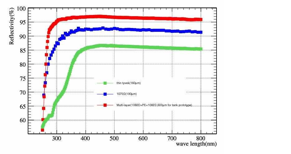
129 5.6. µ µ theta 37 <10GeV 5.55: µ theta( ) ( ) 3 tyvek tyvek tyvek 5.56, tyvek 1082D 275um tyvek 1082D tyvek PE ( ) tyvek( 600 ) tyvek tyvek tyvek tyvek 1082D(275 um) tyvek tyvek tyvek 5.57 tyvek tyvek tyvek 160 ( ) 400nm 85% 86% 1070D tyvek( ) (190 tyvek ) 380nm 92% tyvek (1082D+PE+1082D) 300nm 95% 97% tyvek


130 : tyvek ( tyvek tyvek tyvek ) 5.57: tyvek
 4 a = a min + a i a i a i a i 0.007 0.0025 0.0016 0.001 0.00074 0.00052 0.00035 0.0001 30 m 60 m 80 m 100 m 120 m 140 m 160 m 200 m 5.")
131 5.6. µ : tyvek ( tyvek ) 5.58 tyvek G4dyb 80% tyvek tyvek 96.5% (tyvek ) 97.5% ( tyvek 1%) 98.5% ( tyvek 2%) 99% ( tyvek 2.5%) 4 a = a min + a i a i a i a i m 60 m 80 m 100 m 120 m 140 m 160 m 200 m 5.7: a i ( ) 5 PMT
132 118 5 PMT PMT PMT 60% PMT PMT 20% PMT 6 PMT PMT PMT n PMT n µ µ 22cm 34cm 1.4 µ 5.59 µ 4GeV theta : µ
133 5.6. µ τ tyvek 99% PMT PMT : f(t) = C τ e t t 0 τ ; ( 5.55) τ=68 ns 99% 30 τ 140ns tyvek 5.61 τ tyvek tyvek 99% 140±20m tyvek >80% > 30m χ 2 / ndf 3380 / 938 t ± 1.72 τ ± 0.13 A 2741 ± χ 2 / ndf 3072 / 927 t ± 1.7 τ ± 0.13 A 2710 ± Hit time(ns) Hit time(ns) 5.60: PMT ( PMT PMT) τ=68 ns 2, : tyvek 99% 140 ± 20 m µ µ x=110cm 5.62 µ 1 1 µ ( <200MeV) µ 0.2 GeV
134 : τ tyvek 1 µ 2MeV µ 1 1 µ 5.62 µ 5.63 µ 5.64 PMT µ 15% 20% Mev/cm 15% 5.65 <2.45MeV/cm >2.45MeV/cm 5.66 µ x=110cm
135 5.6. µ TrackLengthIn Water Entries 2000 Mean RMS TrackLength in water (m) 250 ELossInWater Entries 2000 Mean RMS Energy loss in water (GeV) 5.62: µ ( ) ( ) ELossPercmInWater Entries 3548 Mean RMS χ 2 / ndf 314 / 184 Constant ± 12.3 MPV ± Sigma ± Energy loss per cm(mev) ID00p.e. Entries 1774 Mean RMS p.e. number 5.63: µ 5.64: PMT ID00p.e. Entries 1505 Mean RMS χ 2 / ndf / 75 Constant ± 2.07 Mean ± 1.0 Sigma 38.6 ± p.e. number 22 ID00p.e. Entries 269 Mean RMS χ 2 / ndf / 53 Constant ± 8.00 MPV 566 ± 3.9 Sigma ± p.e. number 5.65: µ ( <2.45MeV/cm ) ; : µ ( >=2.45MeV/cm )
136 122 5 Counts data MC h_15mmwater Entries 1742 Mean RMS Number of photoelectron Counts data h_15mmwater Entries 1692 Mean RMS MC Number of photoelectron 5.66: ( PMT PMT ) PMT PMT PMT 0.69 PMT p.e. number data(bottom PMT) MC(bottom PMT) data(side PMT) MC(side PMT) Distance(cm) 5.67: µ PMT µ 5.68 µ 1 1 µ µ <1 ( <0)
137 h_15mmwater Entries 1897 Mean RMS µ TrackLength Entries 9307 Mean RMS TrackLength in water/cm 5.68: µ Counts data MC Number of photoelectron Counts data MC h_15mmwater Entries 1892 Mean RMS Number of photoelectron 5.69: ( PMT PMT) µ tyvek 99% 140±20m µ
138 124 5
139 6 µ PMT PMT PMT tyvek >80% >30 µ tyvek 99% 140 (tyvek >80% > 30 ) µ µ µ µ µ Cerenkov tyvek µ 125
140 126 6
141 [1] W. Pauli, Letter to Tübingen conference, December 4, [2] E, Fermi, Ricerca Scientifica 2, 12(1933). [3] E, Fermi, Z. Phys. 88, 161 (1934); Nuovo Cim. 11, 1 (1934). [4] E.J. Konopinski, Rev. Mod. Phys. 27, 254 (1955). [5] F. Reines, C.L. Cowan, F.B. Harrison, A.D. McGuire and H.W. Kruse, Phys. Rev. 117, 159 (1960). [6] T.D. Lee and C.N. Yang, Phys. Lett. 104, 254 (1956). [7] C.S. Wu, E. Ambler,R.W. Hayward, D.D. Hoppes and R.P. Hudson, Phys. Lett. 105, 1413 (1957). [8] R.P. Feynman and M. Gell-Mann, Phys. Rev. 109,193 (1958); E.C.G. Sudarshan and R.E. Marshak, Phys. Rev. 109, 1860 (1958). [9] L. Landau, Nucl. Phys. 3, 127 (1957); T.D. Lee and C.N. Yang, Phys. Rev (1957). [10] M. Goldhaber, L.Grodzins and A.W. Sunyar, Phys. Rev. 109, 1015 (1958). [11], Nucl. Phys. 22, 579 (1961); S Weinbery, Phys. Rev. Lett. 19, 1264 (1967). [12] P.W. Higgs, Phys. Lett. 12, 132 (1964); Phys. Rev. Lett. 13, 508 (1964); Phys. Rev. 145, 1156 (1966). [13] G. t Hooft, Nucl. Phys. B 33, 173 (1971); Nucl. Phys. B 35, 167 (1971); G. t Hooft and M.J.G. Veltman, Nucl. Phys. B 44, 189 (1972). [14] F.J. Hasert et al., Phys. Lett. B 46, 121 (1973); A.C. Benvenuti et al., Phys. Rev. Lett. 32, 800 (1974); G. Arnison et al., Phys. Lett B 122, 103 (1983). [15] M.L. Perl et al., Phys. Rev. Lett. 35, 1489 (1975). [16] S.W. Herb et al., Phys. Rev. Lett. 39, 252 (1977). [17] F. Abe et al., Phys. Rev. Lett. 74, 2626 (1995); S. Abachi et al., Phys. Rev. Lett. 74, 2632 (1995). 127
Solar Neutrinos: Fluxes
 Solar Neutrinos: Fluxes pp chain Sun shines by : 4 p 4 He + e + + ν e + γ Solar Standard Model Fluxes CNO cycle e + N 13 =0.707MeV He 4 C 1 C 13 p p p p N 15 N 14 He 4 O 15 O 16 e + =0.997MeV O17
 2-2 -1-1 Flux x E ν ( m sec sr GeV ) 1 3 1 2 Honda BGS νµ + νµ νe + νe 1 1 1-2 1-1 1 1 1 Neutrino Energy (GeV) 2.5 Honda ν µ + ν µ ν + e ν e 2.5 BGS ν µ + ν µ ν + e ν e 2. 2. Flux Ratios 1.5 ν e 1.5 ν
Hadronic Tau Decays at BaBar
 Hadronic Tau Decays at BaBar Swagato Banerjee Joint Meeting of Pacific Region Particle Physics Communities (DPF006+JPS006 Honolulu, Hawaii 9 October - 3 November 006 (Page: 1 Hadronic τ decays Only lepton
Dong Liu State Key Laboratory of Particle Detection and Electronics University of Science and Technology of China
 Dong Liu State Key Laboratory of Particle Detection and Electronics University of Science and Technology of China ISSP, Erice, 7 Outline Introduction of BESIII experiment Motivation of the study Data sample
Ηλιακά νετρίνα. Πρόβλημα ηλιακών νετρίνων, ταλαντώσεις.
 Ηλιακά νετρίνα Πρόβλημα ηλιακών νετρίνων, ταλαντώσεις. Αντιδράσεις στο εσωτερικό του Ηλίου (Τυπικό Ηλιακό Μοντέλο) 98,4 % pp pep hep Be B Εικόνα 1Πυρηνικές αντιδράσεις στο κέντρο του ηλίου J.Bacall (2005)
Homework 8 Model Solution Section
 MATH 004 Homework Solution Homework 8 Model Solution Section 14.5 14.6. 14.5. Use the Chain Rule to find dz where z cosx + 4y), x 5t 4, y 1 t. dz dx + dy y sinx + 4y)0t + 4) sinx + 4y) 1t ) 0t + 4t ) sinx
Διερεύνηση ακουστικών ιδιοτήτων Νεκρομαντείου Αχέροντα
 Διερεύνηση ακουστικών ιδιοτήτων Νεκρομαντείου Αχέροντα Βασίλειος Α. Ζαφρανάς Παναγιώτης Σ. Καραμπατζάκης ΠΕΡΙΛΗΨΗ H εργασία αφορά μία σειρά μετρήσεων του χρόνου αντήχησης της υπόγειας κρύπτης του «Νεκρομαντείου»
CorV CVAC. CorV TU317. 1
 30 8 JOURNAL OF VIBRATION AND SHOCK Vol. 30 No. 8 2011 1 2 1 2 2 1. 100044 2. 361005 TU317. 1 A Structural damage detection method based on correlation function analysis of vibration measurement data LEI
Supporting information. An unusual bifunctional Tb-MOF for highly sensing of Ba 2+ ions and remarkable selectivities of CO 2 /N 2 and CO 2 /CH 4
 Electronic Supplementary Material (ESI) for Journal of Materials Chemistry A. This journal is The Royal Society of Chemistry 2015 Supporting information An unusual bifunctional Tb-MOF for highly sensing
SMD Transient Voltage Suppressors
 SMD Transient Suppressors Feature Full range from 0 to 22 series. form 4 to 60V RMS ; 5.5 to 85Vdc High surge current ability Bidirectional clamping, high energy Fast response time
Fused Bis-Benzothiadiazoles as Electron Acceptors
 Fused Bis-Benzothiadiazoles as Electron Acceptors Debin Xia, a,b Xiao-Ye Wang, b Xin Guo, c Martin Baumgarten,*,b Mengmeng Li, b and Klaus Müllen*,b a MIIT Key Laboratory of ritical Materials Technology
Metal Oxide Varistors (MOV) Data Sheet
 Data Sheet") Φ SERIES Metal Oxide Varistors (MOV) Data Sheet Features Wide operating voltage (V ma ) range from 8V to 0V Fast responding to transient over-voltage Large absorbing transient energy capability Low clamping
Φ SERIES Metal Oxide Varistors (MOV) Data Sheet Features Wide operating voltage (V ma ) range from 8V to 0V Fast responding to transient over-voltage Large absorbing transient energy capability Low clamping
Μέθοδοι και Εφαρµογές Πυρηνικής Επιστήµης και Ακτινοφυσικής
 Μέθοδοι και Εφαρµογές Πυρηνικής Επιστήµης και Ακτινοφυσικής Οµάδα Εφαρµοσµένης Πυρηνικής Επιστήµης και Ακτινοφυσικής Σκοπός Έρευνα και Ανάπτυξη στις εφαρµογές της Πυρηνικής Επιστήµης και Ακτινοφυσικής
Οι απόψεις και τα συμπεράσματα που περιέχονται σε αυτό το έγγραφο, εκφράζουν τον συγγραφέα και δεν πρέπει να ερμηνευτεί ότι αντιπροσωπεύουν τις
 Οι απόψεις και τα συμπεράσματα που περιέχονται σε αυτό το έγγραφο, εκφράζουν τον συγγραφέα και δεν πρέπει να ερμηνευτεί ότι αντιπροσωπεύουν τις επίσημες θέσεις των εξεταστών. i ΠΡΟΛΟΓΟΣ ΕΥΧΑΡΙΣΤΙΕΣ Η παρούσα
Υπολογιστική Φυσική Στοιχειωδών Σωματιδίων
 Υπολογιστική Φυσική Στοιχειωδών Σωματιδίων Όρια Πιστότητας (Confidence Limits) 2/4/2014 Υπολογ.Φυσική ΣΣ 1 Τα όρια πιστότητας -Confidence Limits (CL) Tα όρια πιστότητας μιας μέτρησης Μπορεί να αναφέρονται
Mock Exam 7. 1 Hong Kong Educational Publishing Company. Section A 1. Reference: HKDSE Math M Q2 (a) (1 + kx) n 1M + 1A = (1) =
 (1 + kx) n 1M + 1A = (1) =") Mock Eam 7 Mock Eam 7 Section A. Reference: HKDSE Math M 0 Q (a) ( + k) n nn ( )( k) + nk ( ) + + nn ( ) k + nk + + + A nk... () nn ( ) k... () From (), k...() n Substituting () into (), nn ( ) n 76n 76n
Mock Eam 7 Mock Eam 7 Section A. Reference: HKDSE Math M 0 Q (a) ( + k) n nn ( )( k) + nk ( ) + + nn ( ) k + nk + + + A nk... () nn ( ) k... () From (), k...() n Substituting () into (), nn ( ) n 76n 76n
ΠΟΛΥΤΕΧΝΕΙΟ ΚΡΗΤΗΣ ΣΧΟΛΗ ΜΗΧΑΝΙΚΩΝ ΠΕΡΙΒΑΛΛΟΝΤΟΣ
 ΠΟΛΥΤΕΧΝΕΙΟ ΚΡΗΤΗΣ ΣΧΟΛΗ ΜΗΧΑΝΙΚΩΝ ΠΕΡΙΒΑΛΛΟΝΤΟΣ Τομέας Περιβαλλοντικής Υδραυλικής και Γεωπεριβαλλοντικής Μηχανικής (III) Εργαστήριο Γεωπεριβαλλοντικής Μηχανικής TECHNICAL UNIVERSITY OF CRETE SCHOOL of
ΔΙΠΛΩΜΑΤΙΚΗ ΕΡΓΑΣΙΑ. του φοιτητή του Τμήματος Ηλεκτρολόγων Μηχανικών και. Τεχνολογίας Υπολογιστών της Πολυτεχνικής Σχολής του. Πανεπιστημίου Πατρών
 ΠΑΝΕΠΙΣΤΗΜΙΟ ΠΑΤΡΩΝ ΤΜΗΜΑ ΗΛΕΚΤΡΟΛΟΓΩΝ ΜΗΧΑΝΙΚΩΝ ΚΑΙ ΤΕΧΝΟΛΟΓΙΑΣ ΥΠΟΛΟΓΙΣΤΩΝ ΤΟΜΕΑΣ ΣΥΣΤΗΜΑΤΩΝ ΗΛΕΚΤΡΙΚΗΣ ΕΝΕΡΓΕΙΑΣ ΕΡΓΑΣΤΗΡΙΟ ΗΛΕΚΤΡΟΜΗΧΑΝΙΚΗΣ ΜΕΤΑΤΡΟΠΗΣ ΕΝΕΡΓΕΙΑΣ ΔΙΠΛΩΜΑΤΙΚΗ ΕΡΓΑΣΙΑ του φοιτητή του
Fundamental Physical Constants Extensive Listing Relative std. Quantity Symbol Value Unit uncert. u r
 UNIVERSAL speed of light in vacuum c, c 0 299 792 458 m s 1 exact magnetic constant µ 0 4π 10 7 N A 2 = 12.566 370 614... 10 7 N A 2 exact electric constant 1/µ 0 c 2 ɛ 0 8.854 187 817... 10 12 F m 1 exact
6.4 Superposition of Linear Plane Progressive Waves
 .0 - Marine Hydrodynamics, Spring 005 Lecture.0 - Marine Hydrodynamics Lecture 6.4 Superposition of Linear Plane Progressive Waves. Oblique Plane Waves z v k k k z v k = ( k, k z ) θ (Looking up the y-ais
CERN-ACC-SLIDES
 CERN-ACC-SLIDES-2014-0002 13/05/2014 Francesco.Broggi@mi.infn.it Francesco.Broggi@cern.ch RESMM 14 Wroclaw May13 th 2014 Ti5 Nb 3 Sn cable SimpleGeo Plot 1.0x10 12 Activity Decay After Irradiation LHe
Optimizing Microwave-assisted Extraction Process for Paprika Red Pigments Using Response Surface Methodology
 2012 34 2 382-387 http / /xuebao. jxau. edu. cn Acta Agriculturae Universitatis Jiangxiensis E - mail ndxb7775@ sina. com 212018 105 W 42 2 min 0. 631 TS202. 3 A 1000-2286 2012 02-0382 - 06 Optimizing
wave energy Superposition of linear plane progressive waves Marine Hydrodynamics Lecture Oblique Plane Waves:
 3.0 Marine Hydrodynamics, Fall 004 Lecture 0 Copyriht c 004 MIT - Department of Ocean Enineerin, All rihts reserved. 3.0 - Marine Hydrodynamics Lecture 0 Free-surface waves: wave enery linear superposition,
Baryon Studies. Dongliang Zhang (University of Michigan) Hadron2015, Jefferson Lab September 13-18, on behalf of ATLAS Collaboration
 Hadron2015, Jefferson Lab September 13-18, on behalf of ATLAS Collaboration") Λ b Baryon Studies Dongliang Zhang (University of Michigan) on behalf of Collaboration Hadron215, Jefferson Lab September 13-18, 215 Introduction Λ b reconstruction Lifetime measurement Helicity study
Λ b Baryon Studies Dongliang Zhang (University of Michigan) on behalf of Collaboration Hadron215, Jefferson Lab September 13-18, 215 Introduction Λ b reconstruction Lifetime measurement Helicity study
CHAPTER 25 SOLVING EQUATIONS BY ITERATIVE METHODS
 CHAPTER 5 SOLVING EQUATIONS BY ITERATIVE METHODS EXERCISE 104 Page 8 1. Find the positive root of the equation x + 3x 5 = 0, correct to 3 significant figures, using the method of bisection. Let f(x) =
Fundamental Physical Constants Extensive Listing Relative std. Quantity Symbol Value Unit uncert. u r
 UNIVERSAL speed of light in vacuum c, c 0 299 792 458 m s 1 exact magnetic constant µ 0 4π 10 7 N A 2 = 12.566 370 614... 10 7 N A 2 exact electric constant 1/µ 0 c 2 ɛ 0 8.854 187 817... 10 12 F m 1 exact
1 (forward modeling) 2 (data-driven modeling) e- Quest EnergyPlus DeST 1.1. {X t } ARMA. S.Sp. Pappas [4]
![1 (forward modeling) 2 (data-driven modeling) e- Quest EnergyPlus DeST 1.1. {X t } ARMA. S.Sp. Pappas [4]](/thumbs/91/106768733.jpg "1 (forward modeling) 2 (data-driven modeling) e- Quest EnergyPlus DeST 1.1. {X t } ARMA. S.Sp. Pappas [4]") 212 2 ( 4 252 ) No.2 in 212 (Total No.252 Vol.4) doi 1.3969/j.issn.1673-7237.212.2.16 STANDARD & TESTING 1 2 2 (1. 2184 2. 2184) CensusX12 ARMA ARMA TU111.19 A 1673-7237(212)2-55-5 Time Series Analysis
212 2 ( 4 252 ) No.2 in 212 (Total No.252 Vol.4) doi 1.3969/j.issn.1673-7237.212.2.16 STANDARD & TESTING 1 2 2 (1. 2184 2. 2184) CensusX12 ARMA ARMA TU111.19 A 1673-7237(212)2-55-5 Time Series Analysis
Characterization Report
 Characterization Report RF Coaxial Cable Assemblies Raw Cable Type: Temp-Flex 047-2801 RF047-11SP9-11SP9-0305 Test Date: 10 Dec. 2014 RF047-11RP9-11RP9-0305 Test Date: 13 Oct. 2014 RF047-01SP1-01SP1-0305
Current Status of PF SAXS beamlines. 07/23/2014 Nobutaka Shimizu
 Current Status of PF SAXS beamlines 07/23/2014 Nobutaka Shimizu BL-6A Detector SAXS:PILATUS3 1M WAXD:PILATUS 100K Wavelength 1.5Å (Fix) Camera Length 0.25, 0.5, 1.0, 2.0, 2.5 m +WAXD Chamber:0.75, 1.0,
The NOνA Neutrino Experiment
 The NOνA Neutrino Experiment Thomas Coan Southern Methodist University For the NOνA Collaboration 11th ICATPP Villa Olmo, Como 2009 Outline NuMI Off-Axis νe Appearance Experiment Neutrino Physics Motivation
4.4 Superposition of Linear Plane Progressive Waves
 .0 Marine Hydrodynamics, Fall 08 Lecture 6 Copyright c 08 MIT - Department of Mechanical Engineering, All rights reserved..0 - Marine Hydrodynamics Lecture 6 4.4 Superposition of Linear Plane Progressive
Artiste Picasso 9.1. Total Lumen Output: lm. Peak: cd 6862 K CRI: Lumen/Watt. Date: 4/27/2018
 Color Temperature: 62 K Total Lumen Output: 21194 lm Light Quality: CRI:.7 Light Efficiency: 27 Lumen/Watt Peak: 1128539 cd Power: 793 W x: 0.308 y: 0.320 Test: Narrow Date: 4/27/2018 0 Beam Angle 165
(1) Describe the process by which mercury atoms become excited in a fluorescent tube (3)
 Describe the process by which mercury atoms become excited in a fluorescent tube (3)") Q1. (a) A fluorescent tube is filled with mercury vapour at low pressure. In order to emit electromagnetic radiation the mercury atoms must first be excited. (i) What is meant by an excited atom? (1) (ii)
Q1. (a) A fluorescent tube is filled with mercury vapour at low pressure. In order to emit electromagnetic radiation the mercury atoms must first be excited. (i) What is meant by an excited atom? (1) (ii)
ST5224: Advanced Statistical Theory II
 ST5224: Advanced Statistical Theory II 2014/2015: Semester II Tutorial 7 1. Let X be a sample from a population P and consider testing hypotheses H 0 : P = P 0 versus H 1 : P = P 1, where P j is a known
<< 3; -. ; ; ; C? 1 1 B C 4 4 C?. B B; ;? 9= 2 C? 1 1 C 4 4 C?. B
 ! "! #! $ % & ' (# # ) " * +, (! + $ % % # #! -.! # # # / 0 + 1 12 3. 4 5 2 677 8 9 -: ; < = 49 => ==: 4? @9 : 4? ; A 4 B 4 C? =
Enantioselective Organocatalytic Michael Addition of Isorhodanines. to α, β-unsaturated Aldehydes
 Electronic Supplementary Material (ESI) for Organic & Biomolecular Chemistry. This journal is The Royal Society of Chemistry 2016 Enantioselective Organocatalytic Michael Addition of Isorhodanines to α,
Review Test 3. MULTIPLE CHOICE. Choose the one alternative that best completes the statement or answers the question.
 Review Test MULTIPLE CHOICE. Choose the one alternative that best completes the statement or answers the question. Find the exact value of the expression. 1) sin - 11π 1 1) + - + - - ) sin 11π 1 ) ( -
Approximation of distance between locations on earth given by latitude and longitude
 Approximation of distance between locations on earth given by latitude and longitude Jan Behrens 2012-12-31 In this paper we shall provide a method to approximate distances between two points on earth
Laboratory Studies on the Irradiation of Solid Ethane Analog Ices and Implications to Titan s Chemistry
 Laboratory Studies on the Irradiation of Solid Ethane Analog Ices and Implications to Titan s Chemistry 5th Titan Workshop at Kauai, Hawaii April 11-14, 2011 Seol Kim Outer Solar System Model Ices with
Web 論 文. Performance Evaluation and Renewal of Department s Official Web Site. Akira TAKAHASHI and Kenji KAMIMURA
 長 岡 工 業 高 等 専 門 学 校 研 究 紀 要 第 49 巻 (2013) 論 文 Web Department of Electronic Control Engineering, Nagaoka National College of Technology Performance Evaluation and Renewal of Department s Official Web Site
Neutrino experiments and nonstandard interactions
 Neutrino experiments and nonstandard interactions p. 1 Neutrino experiments and nonstandard interactions Omar G. Miranda Romagnoli Cinvestav Neutrino experiments and nonstandard interactions p. 2 Contents
Calculating the propagation delay of coaxial cable
 Your source for quality GNSS Networking Solutions and Design Services! Page 1 of 5 Calculating the propagation delay of coaxial cable The delay of a cable or velocity factor is determined by the dielectric
Cycloaddition of Homochiral Dihydroimidazoles: A 1,3-Dipolar Cycloaddition Route to Optically Active Pyrrolo[1,2-a]imidazoles
![Cycloaddition of Homochiral Dihydroimidazoles: A 1,3-Dipolar Cycloaddition Route to Optically Active Pyrrolo[1,2-a]imidazoles](/thumbs/89/100111450.jpg "Cycloaddition of Homochiral Dihydroimidazoles: A 1,3-Dipolar Cycloaddition Route to Optically Active Pyrrolo[1,2-a]imidazoles") X-Ray crystallographic data tables for paper: Supplementary Material (ESI) for Organic & Biomolecular Chemistry Cycloaddition of Homochiral Dihydroimidazoles: A 1,3-Dipolar Cycloaddition Route to Optically
X-Ray crystallographic data tables for paper: Supplementary Material (ESI) for Organic & Biomolecular Chemistry Cycloaddition of Homochiral Dihydroimidazoles: A 1,3-Dipolar Cycloaddition Route to Optically
Study on Re-adhesion control by monitoring excessive angular momentum in electric railway traction
 () () Study on e-adhesion control by monitoring excessive angular momentum in electric railway traction Takafumi Hara, Student Member, Takafumi Koseki, Member, Yutaka Tsukinokizawa, Non-member Abstract
the total number of electrons passing through the lamp.
 1. A 12 V 36 W lamp is lit to normal brightness using a 12 V car battery of negligible internal resistance. The lamp is switched on for one hour (3600 s). For the time of 1 hour, calculate (i) the energy
2.1
 181 8588 2 21 1 e-mail: sekig@th.nao.ac.jp 1. G ab kt ab, (1) k 8pGc 4, G c 2. 1 2.1 308 2009 5 3 1 2) ( ab ) (g ab ) (K ab ) 1 2.2 3 1 (g ab, K ab ) 1 t a S n a a b a 2.3 a b i (t a ) 2 1 2.4 1 g ab ab
Math221: HW# 1 solutions
 Math: HW# solutions Andy Royston October, 5 7.5.7, 3 rd Ed. We have a n = b n = a = fxdx = xdx =, x cos nxdx = x sin nx n sin nxdx n = cos nx n = n n, x sin nxdx = x cos nx n + cos nxdx n cos n = + sin
Type 947D Polypropylene, High Energy Density, DC Link Capacitors
 Type 947D series uses the most advanced metallized film technology for long life and high reliability in DC Link applications. This series combines high capacitance and very high ripple current capability
..,..,.. ! " # $ % #! & %
 ..,..,.. - -, - 2008 378.146(075.8) -481.28 73 69 69.. - : /..,..,... : - -, 2008. 204. ISBN 5-98298-269-5. - -,, -.,,, -., -. - «- -»,. 378.146(075.8) -481.28 73 -,..,.. ISBN 5-98298-269-5..,..,.., 2008,
Tsunami Runup and Inundation Simulation in Malaysia Including the Role of Mangroves
 Tsunami Runup and Inundation Simulation in Malaysia Including the Role of Mangroves Teh Su Yean, Koh Hock Lye, Philip Liu, Ahmad Izani Md Ismail and 3 Lee Hooi Ling School of Mathematical Sciences, Universiti
LIGHT UNFLAVORED MESONS (S = C = B = 0)
") LIGHT UNFLAVORED MESONS (S = C = B = 0) For I = 1 (π, b, ρ, a): ud, (uu dd)/ 2, du; for I = 0 (η, η, h, h, ω, φ, f, f ): c 1 (uu + d d) + c 2 (s s) π ± I G (J P ) = 1 (0 ) Mass m = 139.57018 ± 0.00035
LIGHT UNFLAVORED MESONS (S = C = B = 0) For I = 1 (π, b, ρ, a): ud, (uu dd)/ 2, du; for I = 0 (η, η, h, h, ω, φ, f, f ): c 1 (uu + d d) + c 2 (s s) π ± I G (J P ) = 1 (0 ) Mass m = 139.57018 ± 0.00035
measured by ALICE in pp, p-pb and Pb-Pb collisions at the LHC
 Σ(85) Ξ(5) Production of and measured by ALICE in pp, ppb and PbPb collisions at the LHC for the ALICE Collaboration Pusan National University, OREA Quark Matter 7 in Chicago 7.. QM7 * suppressed, no suppression
Other Test Constructions: Likelihood Ratio & Bayes Tests
 Other Test Constructions: Likelihood Ratio & Bayes Tests Side-Note: So far we have seen a few approaches for creating tests such as Neyman-Pearson Lemma ( most powerful tests of H 0 : θ = θ 0 vs H 1 :
Nuclear Physics 5. Name: Date: 8 (1)
") Name: Date: Nuclear Physics 5. A sample of radioactive carbon-4 decays into a stable isotope of nitrogen. As the carbon-4 decays, the rate at which the amount of nitrogen is produced A. decreases linearly
Name: Date: Nuclear Physics 5. A sample of radioactive carbon-4 decays into a stable isotope of nitrogen. As the carbon-4 decays, the rate at which the amount of nitrogen is produced A. decreases linearly
UDZ Swirl diffuser. Product facts. Quick-selection. Swirl diffuser UDZ. Product code example:
 UDZ Swirl diffuser Swirl diffuser UDZ, which is intended for installation in a ventilation duct, can be used in premises with a large volume, for example factory premises, storage areas, superstores, halls,
No. 7 Modular Machine Tool & Automatic Manufacturing Technique. Jul TH166 TG659 A
 7 2016 7 No. 7 Modular Machine Tool & Automatic Manufacturing Technique Jul. 2016 1001-2265 2016 07-0122 - 05 DOI 10. 13462 /j. cnki. mmtamt. 2016. 07. 035 * 100124 TH166 TG659 A Precision Modeling and
Conductivity Logging for Thermal Spring Well
 /.,**. 25 +,1- **-- 0/2,,,1- **-- 0/2, +,, +/., +0 /,* Conductivity Logging for Thermal Spring Well Koji SATO +, Tadashi TAKAYA,, Tadashi CHIBA, + Nihon Chika Kenkyuusho Co. Ltd., 0/2,, Hongo, Funabashi,
Ηλιακά νετρίνα. Εικόνα 1 Πυρηνικές αντιδράσεις στο κέντρο του ηλίου. * σ ve : 9.3*10-45 cm 2 (E/Mev) 2
 2") Ηλιακά νετρίνα. Γνωρίζουμε ότι ενέργεια που ακτινοβολεί ο ήλιος, παράγεται από θερμοπυρηνικές αντιδράσεις στον πυρήνα του ηλίου. Στα προϊόντα των αντιδράσεων περιλαμβάνεται μεγάλος αριθμός νετρίνων. Μπορούμε
Ηλιακά νετρίνα. Γνωρίζουμε ότι ενέργεια που ακτινοβολεί ο ήλιος, παράγεται από θερμοπυρηνικές αντιδράσεις στον πυρήνα του ηλίου. Στα προϊόντα των αντιδράσεων περιλαμβάνεται μεγάλος αριθμός νετρίνων. Μπορούμε
ΤΕΧΝΟΛΟΓΙΚΟ ΠΑΝΕΠΙΣΤΗΜΙΟ ΚΥΠΡΟΥ ΣΧΟΛΗ ΓΕΩΤΕΧΝΙΚΩΝ ΕΠΙΣΤΗΜΩΝ ΚΑΙ ΔΙΑΧΕΙΡΙΣΗΣ ΠΕΡΙΒΑΛΛΟΝΤΟΣ. Πτυχιακή εργασία
 ΤΕΧΝΟΛΟΓΙΚΟ ΠΑΝΕΠΙΣΤΗΜΙΟ ΚΥΠΡΟΥ ΣΧΟΛΗ ΓΕΩΤΕΧΝΙΚΩΝ ΕΠΙΣΤΗΜΩΝ ΚΑΙ ΔΙΑΧΕΙΡΙΣΗΣ ΠΕΡΙΒΑΛΛΟΝΤΟΣ Πτυχιακή εργασία ΚΑΤΑΣΚΕΥΗ ΦΩΤΟΑΝΤΙΔΡΑΣΤΗΡΑ (UV) ΓΙΑ ΠΕΡΙΒΑΛΛΟΝΤΙΚΕΣ ΕΦΑΡΜΟΓΕΣ Δημήτρης Δημητρίου Λεμεσός 2015
for fracture orientation and fracture density on physical model data
 AVAZ inversion for fracture orientation and fracture density on physical model data Faranak Mahmoudian Gary Margrave CREWES Tech talk, February 0 th, 0 Objective Inversion of prestack PP amplitudes (different
Te chnical Data Catalog
 Te chnical Data Catalog 50 khz 1 kw 50 khz AE Power rating: 1 kwrms @ 2% duty cycle 7x28mm (1.13") PZT/L Active Area: 45cm 2 Urethane Window Beamwidth: -3dB: 19-6dB: 27 db: 34 Directivity Index: 18.9 Frequency
Magnetised Iron Neutrino Detector. (MIND) at a Neutrino Factory. Neutrino GDR Meeting, Paris, 29 April 2010
 at a Neutrino Factory. Neutrino GDR Meeting, Paris, 29 April 2010") Magnetised Iron Neutrino Detector (MIND) at a Neutrino Factory, Paul Soler*, Anselmo Cervera, Andrew Laing, Justo Martín-Albo Neutrino mixing Weak eigenstates do not have to coincide with mass eigenstates
Magnetised Iron Neutrino Detector (MIND) at a Neutrino Factory, Paul Soler*, Anselmo Cervera, Andrew Laing, Justo Martín-Albo Neutrino mixing Weak eigenstates do not have to coincide with mass eigenstates
Πανεπιστήμιο Κρήτης, Τμήμα Επιστήμης Υπολογιστών Άνοιξη 2009. HΥ463 - Συστήματα Ανάκτησης Πληροφοριών Information Retrieval (IR) Systems
 Systems") Πανεπιστήμιο Κρήτης, Τμήμα Επιστήμης Υπολογιστών Άνοιξη 2009 HΥ463 - Συστήματα Ανάκτησης Πληροφοριών Information Retrieval (IR) Systems Στατιστικά Κειμένου Text Statistics Γιάννης Τζίτζικας άλ ιάλεξη :
Πανεπιστήμιο Κρήτης, Τμήμα Επιστήμης Υπολογιστών Άνοιξη 2009 HΥ463 - Συστήματα Ανάκτησης Πληροφοριών Information Retrieval (IR) Systems Στατιστικά Κειμένου Text Statistics Γιάννης Τζίτζικας άλ ιάλεξη :
IL - 13 /IL - 18 ELISA PCR RT - PCR. IL - 13 IL - 18 mrna. 13 IL - 18 mrna IL - 13 /IL Th1 /Th2
 344 IL - 13 /IL - 18 1 2 1 2 1 2 1 2 1 2 3 1 2 13 18 IL - 13 /IL - 18 10% / OVA /AL OH 3 5% 16 ~ 43 d 44 d ELISA BALF IL - 13 IL - 18 PCR RT - PCR IL - 13 IL - 18 mrna IL - 13 mrna 0. 01 IL - 18 mrna 0.
Study on the Strengthen Method of Masonry Structure by Steel Truss for Collapse Prevention
 33 2 2011 4 Vol. 33 No. 2 Apr. 2011 1002-8412 2011 02-0096-08 1 1 1 2 3 1. 361005 3. 361004 361005 2. 30 TU746. 3 A Study on the Strengthen Method of Masonry Structure by Steel Truss for Collapse Prevention
Answers to practice exercises
 Answers to practice exercises Chapter Exercise (Page 5). 9 kg 2. 479 mm. 66 4. 565 5. 225 6. 26 7. 07,70 8. 4 9. 487 0. 70872. $5, Exercise 2 (Page 6). (a) 468 (b) 868 2. (a) 827 (b) 458. (a) 86 kg (b)
IV. ANHANG 179. Anhang 178
 Anhang 178 IV. ANHANG 179 1. Röntgenstrukturanalysen (Tabellen) 179 1.1. Diastereomer A (Diplomarbeit) 179 1.2. Diastereomer B (Diplomarbeit) 186 1.3. Aldoladdukt 5A 193 1.4. Aldoladdukt 13A 200 1.5. Aldoladdukt
Το άτομο του Υδρογόνου
 Το άτομο του Υδρογόνου Δυναμικό Coulomb Εξίσωση Schrödinger h e (, r, ) (, r, ) E (, r, ) m ψ θφ r ψ θφ = ψ θφ Συνθήκες ψ(, r θφ, ) = πεπερασμένη ψ( r ) = 0 ψ(, r θφ, ) =ψ(, r θφ+, ) π Επιτρεπτές ενέργειες
þÿ ³¹µ¹½ º±¹ ±ÃÆ»µ¹± ÃÄ ÇÎÁ
 Neapolis University HEPHAESTUS Repository School of Economic Sciences and Business http://hephaestus.nup.ac.cy Master Degree Thesis 2014 þÿ ³¹µ¹½ º±¹ ±ÃÆ»µ¹± ÃÄ ÇÎÁ þÿµá³±ã ±Â Äɽ ½ à º ¼µ ɽ : Georgiou,
ΜΕΛΕΤΗ ΤΗΣ ΗΛΕΚΤΡΟΝΙΚΗΣ ΣΥΝΤΑΓΟΓΡΑΦΗΣΗΣ ΚΑΙ Η ΔΙΕΡΕΥΝΗΣΗ ΤΗΣ ΕΦΑΡΜΟΓΗΣ ΤΗΣ ΣΤΗΝ ΕΛΛΑΔΑ: Ο.Α.Ε.Ε. ΠΕΡΙΦΕΡΕΙΑ ΠΕΛΟΠΟΝΝΗΣΟΥ ΚΑΣΚΑΦΕΤΟΥ ΣΩΤΗΡΙΑ
 ΠΑΝΕΠΙΣΤΗΜΙΟ ΠΕΙΡΑΙΩΣ ΠΡΟΓΡΑΜΜΑ ΜΕΤΑΠΤΥΧΙΑΚΩΝ ΣΠΟΥΔΩΝ ΔΙΟΙΚΗΣΗ ΤΗΣ ΥΓΕΙΑΣ ΤΕΙ ΠΕΙΡΑΙΑ ΜΕΛΕΤΗ ΤΗΣ ΗΛΕΚΤΡΟΝΙΚΗΣ ΣΥΝΤΑΓΟΓΡΑΦΗΣΗΣ ΚΑΙ Η ΔΙΕΡΕΥΝΗΣΗ ΤΗΣ ΕΦΑΡΜΟΓΗΣ ΤΗΣ ΣΤΗΝ ΕΛΛΑΔΑ: Ο.Α.Ε.Ε. ΠΕΡΙΦΕΡΕΙΑ ΠΕΛΟΠΟΝΝΗΣΟΥ
상대론적고에너지중이온충돌에서 제트입자와관련된제동복사 박가영 인하대학교 윤진희교수님, 권민정교수님
 상대론적고에너지중이온충돌에서 제트입자와관련된제동복사 박가영 인하대학교 윤진희교수님, 권민정교수님 Motivation Bremsstrahlung is a major rocess losing energies while jet articles get through the medium. BUT it should be quite different from low energy
k A = [k, k]( )[a 1, a 2 ] = [ka 1,ka 2 ] 4For the division of two intervals of confidence in R +
[a 1, a 2 ] = [ka 1,ka 2 ] 4For the division of two intervals of confidence in R +](/thumbs/73/69566903.jpg "k A = [k, k]( )[a 1, a 2 ] = [ka 1,ka 2 ] 4For the division of two intervals of confidence in R +") Chapter 3. Fuzzy Arithmetic 3- Fuzzy arithmetic: ~Addition(+) and subtraction (-): Let A = [a and B = [b, b in R If x [a and y [b, b than x+y [a +b +b Symbolically,we write A(+)B = [a (+)[b, b = [a +b
Chapter 3. Fuzzy Arithmetic 3- Fuzzy arithmetic: ~Addition(+) and subtraction (-): Let A = [a and B = [b, b in R If x [a and y [b, b than x+y [a +b +b Symbolically,we write A(+)B = [a (+)[b, b = [a +b
Te chnical Data Catalog
 Te chnical Data Catalog 50 khz 1 kw 50 khz AE Power rating: 1 kwrms @ 2% duty cycle 7x28mm (1.13") PZT/L Active Area: 45cm 2 Urethane Window Beamwidth: -3dB: 19-6dB: 27 db: 34 Directivity Index: 18.9 Frequency
Monolithic Crystal Filters (M.C.F.)
") Monolithic Crystal Filters (M.C.F.) MCF (MONOLITHIC CRYSTAL FILTER) features high quality quartz resonators such as sharp cutoff characteristics, low loss, good inter-modulation and high stability over
Monolithic Crystal Filters (M.C.F.) MCF (MONOLITHIC CRYSTAL FILTER) features high quality quartz resonators such as sharp cutoff characteristics, low loss, good inter-modulation and high stability over
derivation of the Laplacian from rectangular to spherical coordinates
 derivation of the Laplacian from rectangular to spherical coordinates swapnizzle 03-03- :5:43 We begin by recognizing the familiar conversion from rectangular to spherical coordinates (note that φ is used
Inverse trigonometric functions & General Solution of Trigonometric Equations. ------------------ ----------------------------- -----------------
 Inverse trigonometric functions & General Solution of Trigonometric Equations. 1. Sin ( ) = a) b) c) d) Ans b. Solution : Method 1. Ans a: 17 > 1 a) is rejected. w.k.t Sin ( sin ) = d is rejected. If sin
 Problem 7.19 Ignoring reflection at the air soil boundary, if the amplitude of a 3-GHz incident wave is 10 V/m at the surface of a wet soil medium, at what depth will it be down to 1 mv/m? Wet soil is
Ηλεκτρικές δοκιµές σε καλώδια µέσης τάσης - ιαδικασίες επαλήθευσης και υπολογισµού αβεβαιότητας ΙΠΛΩΜΑΤΙΚΗ ΕΡΓΑΣΙΑ
 ΕΘΝΙΚΟ ΜΕΤΣΟΒΙΟ ΠΟΛΥΤΕΧΝΕΙΟ ΣΧΟΛΗ ΗΛΕΚΤΡΟΛΟΓΩΝ ΜΗΧΑΝΙΚΩΝ ΚΑΙ ΜΗΧΑΝΙΚΩΝ ΥΠΟΛΟΓΙΣΤΩΝ ΤΟΜΕΑΣ ΗΛΕΚΤΡΙΚΗΣ ΙΣΧΥΟΣ ΕΡΓΑΣΤΗΡΙΟ ΥΨΗΛΩΝ ΤΑΣΕΩΝ Ηλεκτρικές δοκιµές σε καλώδια µέσης τάσης - ιαδικασίες επαλήθευσης και
Chapter 22 - Heat Engines, Entropy, and the Second Law of Thermodynamics
 apter - Heat Engines, Entropy, and te Seond Law o ermodynamis.1 (a).0 J e 0.069 4 or 6.94% 60 J (b) 60 J.0 J J. e eat to melt 1.0 g o Hg is 4 ml 1 10 kg 1.18 10 J kg 177 J e energy absorbed to reeze 1.00
Conjoint. The Problems of Price Attribute by Conjoint Analysis. Akihiko SHIMAZAKI * Nobuyuki OTAKE
 Conjoint Conjoint The Problems of Price Attribute by Conjoint Analysis Akihiko SHIMAZAKI * Nobuyuki OTAKE +, Conjoint - Conjoint. / 0 PSM Price Sensitivity Measurement Conjoint 1 2 + Conjoint Luce and
Fourier Analysis of Waves
 Exercises for the Feynman Lectures on Physics by Richard Feynman, Et Al. Chapter 36 Fourier Analysis of Waves Detailed Work by James Pate Williams, Jr. BA, BS, MSwE, PhD From Exercises for the Feynman
Fundamental Physical Constants Complete Listing Relative std. Quantity Symbol Value Unit uncert. u r
 UNIVERSAL speed of light in vacuum c, c 0 299 792 458 m s 1 (exact) magnetic constant µ 0 4π 10 7 NA 2 = 12.566 370614... 10 7 NA 2 (exact) electric constant 1/µ 0 c 2 ε 0 8.854 187 817... 10 12 Fm 1 (exact)
Homework 3 Solutions
 Homework 3 Solutions Igor Yanovsky (Math 151A TA) Problem 1: Compute the absolute error and relative error in approximations of p by p. (Use calculator!) a) p π, p 22/7; b) p π, p 3.141. Solution: For
Areas and Lengths in Polar Coordinates
 Kiryl Tsishchanka Areas and Lengths in Polar Coordinates In this section we develop the formula for the area of a region whose boundary is given by a polar equation. We need to use the formula for the
Reaction of a Platinum Electrode for the Measurement of Redox Potential of Paddy Soil
 J. Jpn. Soc. Soil Phys. No. +*0, p.- +*,**1 Eh * ** Reaction of a Platinum Electrode for the Measurement of Redox Potential of Paddy Soil Daisuke MURAKAMI* and Tatsuaki KASUBUCHI** * The United Graduate
14.5mm 14.5mm
 This article has been accepted for publication in a future issue of this journal, but has not been fully edited. Content may change prior to final publication. Citation information: DOI 1.119/JETCAS.218.289582,
Rectangular Polar Parametric
 Harold s Precalculus Rectangular Polar Parametric Cheat Sheet 15 October 2017 Point Line Rectangular Polar Parametric f(x) = y (x, y) (a, b) Slope-Intercept Form: y = mx + b Point-Slope Form: y y 0 = m
Data Sheet High Reliability Glass Epoxy Multi-layer Materials (High Tg & Low CTE type) Laminate R-1755V Prepreg R-1650V
 Laminate R-1755V Prepreg R-1650V") Data Sheet High Reliability Glass Epoxy Multi-layer Materials (High Tg & Low CTE type) Laminate R-1755V Prepreg R-1650V Nov. 2015 No.15111336 Specification / Laminate R-1755V No.; 15111336-1 Property Units
Data Sheet High Reliability Glass Epoxy Multi-layer Materials (High Tg & Low CTE type) Laminate R-1755V Prepreg R-1650V Nov. 2015 No.15111336 Specification / Laminate R-1755V No.; 15111336-1 Property Units
LEPTONS. Mass m = ( ± ) 10 6 u Mass m = ± MeV me + m e
 10 6 u Mass m = ± MeV me + m e") LEPTONS e J = 1 2 Mass m = (548.5799110 ± 0.0000012) 10 6 u Mass m = 0.510998902 ± 0.000000021 MeV me + m e /m < 8 10 9, CL = 90% qe + + q / e e < 4 10 8 Magnetic moment µ =1.001159652187 ± 0.000000000004
LEPTONS e J = 1 2 Mass m = (548.5799110 ± 0.0000012) 10 6 u Mass m = 0.510998902 ± 0.000000021 MeV me + m e /m < 8 10 9, CL = 90% qe + + q / e e < 4 10 8 Magnetic moment µ =1.001159652187 ± 0.000000000004
Simplex Crossover for Real-coded Genetic Algolithms
 Technical Papers GA Simplex Crossover for Real-coded Genetic Algolithms 47 Takahide Higuchi Shigeyoshi Tsutsui Masayuki Yamamura Interdisciplinary Graduate school of Science and Engineering, Tokyo Institute
ΜΑΘΗΜΑΤΙΚΗ ΠΡΟΣΟΜΟΙΩΣΗ ΤΗΣ ΔΥΝΑΜΙΚΗΣ ΤΟΥ ΕΔΑΦΙΚΟΥ ΝΕΡΟΥ ΣΤΗΝ ΠΕΡΙΠΤΩΣΗ ΑΡΔΕΥΣΗΣ ΜΕ ΥΠΟΓΕΙΟΥΣ ΣΤΑΛΑΚΤΗΦΟΡΟΥΣ ΣΩΛΗΝΕΣ ΣΕ ΔΙΑΣΤΡΩΜΕΝΑ ΕΔΑΦΗ
 ΓΕΩΠΟΝΙΚΟ ΠΑΝΕΠΙΣΤΗΜΙΟ ΑΘΗΝΩΝ ΤΜΗΜΑ ΑΞΙΟΠΟΙΗΣΗΣ ΦΥΣΙΚΩΝ ΠΟΡΩΝ ΚΑΙ ΓΕΩΡΓΙΚΗΣ ΜΗΧΑΝΙΚΗΣ ΠΡΟΓΡΑΜΜΑ ΜΕΤΑΠΤΥΧΙΑΚΩΝ ΣΠΟΥΔΩΝ ΑΕΙΦΟΡΙΚΗ ΔΙΑΧΕΙΡΙΣΗ ΥΔΑΤΙΚΩΝ ΠΟΡΩΝ Δημήτριος Πάντζαλης Πτυχιούχος Γεωπόνος Α.Π.Θ.
ΘΕΡΜΟΚΗΠΙΑΚΕΣ ΚΑΛΛΙΕΡΓΕΙΕΣ ΕΚΤΟΣ ΕΔΑΦΟΥΣ ΘΡΕΠΤΙΚΑ ΔΙΑΛΥΜΑΤΑ
 ΘΕΡΜΟΚΗΠΙΑΚΕΣ ΚΑΛΛΙΕΡΓΕΙΕΣ ΕΚΤΟΣ ΕΔΑΦΟΥΣ ΘΡΕΠΤΙΚΑ ΔΙΑΛΥΜΑΤΑ Θρεπτικό διάλυμα Είναι ένα αραιό υδατικό διάλυμα όλων των θρεπτικών στοιχείων που είναι απαραίτητα για τα φυτά, τα οποία βρίσκονται διαλυμένα
ΧΑΡΑΚΤΗΡΙΣΜΟΣ ΦΑΣΕΩΝ ΣΙΔΗΡΟΥ ΣΕ ΔΕΙΓΜΑΤΑ ΟΡΥΚΤΩΝ ΑΠΟ ΤΟ ΥΠΟΘΑΛΑΣΣΙΟ ΗΦΑΙΣΤΕΙΟ ΚΟΛΟΥΜΠΟ (ΣΑΝΤΟΡΙΝΗ) ΜΕ ΧΡΗΣΗ ΑΚΤΙΝΟΒΟΛΙΑΣ ΣΥΓΧΡΟΤΡΟΥ
 ΜΕ ΧΡΗΣΗ ΑΚΤΙΝΟΒΟΛΙΑΣ ΣΥΓΧΡΟΤΡΟΥ") ΔΙΠΛΩΜΑΤΙΚΗ ΕΡΓΑΣΙΑ ΧΑΡΑΚΤΗΡΙΣΜΟΣ ΦΑΣΕΩΝ ΣΙΔΗΡΟΥ ΣΕ ΔΕΙΓΜΑΤΑ ΟΡΥΚΤΩΝ ΑΠΟ ΤΟ ΥΠΟΘΑΛΑΣΣΙΟ ΗΦΑΙΣΤΕΙΟ ΚΟΛΟΥΜΠΟ (ΣΑΝΤΟΡΙΝΗ) ΜΕ ΧΡΗΣΗ ΑΚΤΙΝΟΒΟΛΙΑΣ ΣΥΓΧΡΟΤΡΟΥ ΒΑΣΣΑΛΟΣ ΚΩΝΣΤΑΝΤΙΝΟΣ 200500022 ΕΠΙΒΛΕΠΩΝ ΜΕΡΤΖΙΜΕΚΗΣ
ΔΙΠΛΩΜΑΤΙΚΗ ΕΡΓΑΣΙΑ ΧΑΡΑΚΤΗΡΙΣΜΟΣ ΦΑΣΕΩΝ ΣΙΔΗΡΟΥ ΣΕ ΔΕΙΓΜΑΤΑ ΟΡΥΚΤΩΝ ΑΠΟ ΤΟ ΥΠΟΘΑΛΑΣΣΙΟ ΗΦΑΙΣΤΕΙΟ ΚΟΛΟΥΜΠΟ (ΣΑΝΤΟΡΙΝΗ) ΜΕ ΧΡΗΣΗ ΑΚΤΙΝΟΒΟΛΙΑΣ ΣΥΓΧΡΟΤΡΟΥ ΒΑΣΣΑΛΟΣ ΚΩΝΣΤΑΝΤΙΝΟΣ 200500022 ΕΠΙΒΛΕΠΩΝ ΜΕΡΤΖΙΜΕΚΗΣ
Matrices and Determinants
 Matrices and Determinants SUBJECTIVE PROBLEMS: Q 1. For what value of k do the following system of equations possess a non-trivial (i.e., not all zero) solution over the set of rationals Q? x + ky + 3z
Supplementary Materials for Evolutionary Multiobjective Optimization Based Multimodal Optimization: Fitness Landscape Approximation and Peak Detection
 IEEE TRANSACTIONS ON EVOLUTIONARY COMPUTATION, VOL. XX, NO. X, XXXX XXXX Supplementary Materials for Evolutionary Multiobjective Optimization Based Multimodal Optimization: Fitness Landscape Approximation
Table S1. Summary of data collections and structure refinements for crystals 1Rb-1h, 1Rb-2h, and 1Rb-4h.
 Supporting Information [NH 3 CH 3 ] [In SbS 9 SH]: A novel methylamine-directed indium thioantimonate with Rb + ion-exchange property Kai-Yao Wang a,b, Mei-Ling Feng a, Jian-Rong Li a and Xiao-Ying Huang
VSC STEADY2STATE MOD EL AND ITS NONL INEAR CONTROL OF VSC2HVDC SYSTEM VSC (1. , ; 2. , )
") 22 1 2002 1 Vol. 22 No. 1 Jan. 2002 Proceedings of the CSEE ν 2002 Chin. Soc. for Elec. Eng. :025828013 (2002) 0120017206 VSC 1, 1 2, (1., 310027 ; 2., 250061) STEADY2STATE MOD EL AND ITS NONL INEAR CONTROL
22 1 2002 1 Vol. 22 No. 1 Jan. 2002 Proceedings of the CSEE ν 2002 Chin. Soc. for Elec. Eng. :025828013 (2002) 0120017206 VSC 1, 1 2, (1., 310027 ; 2., 250061) STEADY2STATE MOD EL AND ITS NONL INEAR CONTROL
38 Te(OH) 6 2NH 4 H 2 PO 4 (NH 4 ) 2 HPO 4
 6 2NH 4 H 2 PO 4 (NH 4 ) 2 HPO 4") Fig. A-1-1. Te(OH) NH H PO (NH ) HPO (TAAP). Projection of the crystal structure along the b direction [Ave]. 9 1. 7.5 ( a a )/ a [1 ] ( b b )/ b [1 ] 5..5 1.5 1 1.5 ( c c )/ c [1 ].5 1. 1.5. Angle β 1.
Fig. A-1-1. Te(OH) NH H PO (NH ) HPO (TAAP). Projection of the crystal structure along the b direction [Ave]. 9 1. 7.5 ( a a )/ a [1 ] ( b b )/ b [1 ] 5..5 1.5 1 1.5 ( c c )/ c [1 ].5 1. 1.5. Angle β 1.
Neutralization E#ects of Acidity of Rain by Cover Plants on Slope Land
 J. Jpn. Soc. Soil Phys. No. 33, p.2/ 3.,**/ * * * ** Neutralization E#ects of Acidity of Rain by Cover Plants on Slope Land Tadashi ADACHI*, Yoko OKI*, Akihiro NAGAI* and Shogo NAKATSUKASA** * Faculty
ΤΕΧΝΟΛΟΓΙΚΟ ΠΑΝΕΠΙΣΤΗΜΙΟ ΚΥΠΡΟΥ ΣΧΟΛΗ ΓΕΩΤΕΧΝΙΚΩΝ ΕΠΙΣΤΗΜΩΝ ΚΑΙ ΔΙΑΧΕΙΡΙΣΗΣ ΠΕΡΙΒΑΛΛΟΝΤΟΣ. Πτυχιακή εργασία
 ΤΕΧΝΟΛΟΓΙΚΟ ΠΑΝΕΠΙΣΤΗΜΙΟ ΚΥΠΡΟΥ ΣΧΟΛΗ ΓΕΩΤΕΧΝΙΚΩΝ ΕΠΙΣΤΗΜΩΝ ΚΑΙ ΔΙΑΧΕΙΡΙΣΗΣ ΠΕΡΙΒΑΛΛΟΝΤΟΣ Πτυχιακή εργασία ΜΑΘΗΜΑΤΙΚΟΙ ΑΛΓΟΡΙΘΜΟΙ ΓΙΑ ΑΝΑΛΥΣΗ ΠΙΣΤΟΠΟΙΗΤΙΚΩΝ ΕΝΕΡΓΕΙΑΚΗΣ ΑΠΟΔΟΣΗΣ ΚΤΙΡΙΩΝ Εβελίνα Θεμιστοκλέους