CONTINUUM MECHANICS. e 3. x e 2 O e 1. - volume / area V 0, V / A 0,A - base vectors { e 1, e 2, e 3 } - position vector x 0, x

Transcript

1 INTRODUCTION

2 CONTINUUM MECHANICS V 0 A 0 u V A x 0 e 3 x e 2 O e 1 - volume / area V 0, V / A 0,A - base vectors { e 1, e 2, e 3 } - position vector x 0, x - displacement vector u - strains ε kl = 1 2 (u k,l + u l,k ) - compatibility relations - equilibrium equations σ ij,j + ρq i = 0 ; σ ij = σ ji - density ρ - load/mass q i - boundary conditions p i = σ ij n j - material model σ ij = N ij (ε kl )

3 MATERIAL BEHAVIOR σ ε t 1 t 2 t t 1 t 2 t σ ε t 1 t 2 t t 1 t 2 t σ ε t 1 t 2 t t 1 t 2 t

4 STRESS-STRAIN CURVES σ σ σ σ ε ε ε ε

5 FRACTURE

6 FRACTURE MECHANICS (Source: internet) questions : when crack growth? ( crack growth criteria) crack growth rate? residual strength? life time? inspection frequency? repair required? fields of science : material science and chemistry theoretical and numerical mathematics experimental and theoretical mechanics

7 OVERVIEW OF FRACTURE MECHANICS LEFM (Linear Elastic Fracture Mechanics) energy balance crack tip stresses SSY (Small Scale Yielding) DFM (Dynamic Fracture Mechanics) NLFM (Non-Linear Fracture Mechanics) EPFM (Elasto-Plastic Fracture Mechanics) Numerical methods : EEM / BEM Fatigue (HCF / LCF) CDM (Continuum Damage Mechanics) Micro mechanics micro-cracks (intra grain) voids (intra grain) cavities at grain boundaries rupture & disentangling of molecules rupture of atomic bonds dislocation slip

8 EXPERIMENTAL FRACTURE MECHANICS (Source: Internet)

9 LINEAR ELASTIC FRACTURE MECHANICS

10 DYNAMIC FRACTURE MECHANICS

11 NONLINEAR FRACTURE MECHANICS CTOD J-integral

12 NUMERICAL TECHNIQUES

13 FATIGUE

14 OBJECTIVES Insight in : crack growth mechanisms brittle / ductile energy balance crack tip stresses crack growth direction plastic crack tip zone crack growth speed nonlinear fracture mechanics numerical methods fatigue

15

16 FRACTURE MECHANICS

17 FRACTURE MECHANISMS shear fracture cleavage fracture fatigue fracture crazing de-adhesion

18 SHEARING dislocations voids crack dimples load direction

19 CLEAVAGE intra-granulair inter-granulair intra-granular HCP-, BCC-crystal T low ε high 3D-stress state inter-granular weak grain boundary environment (H 2 ) T high

20 FATIGUE clam shell pattern striations

21 CRAZING (Source: Internet) stress whitening crazing materials : PS, PMMA

22 DUCTILE - BRITTLE BEHAVIOR σ ABS, nylon, PC PE, PTFE ε (%) surface energy : γ [Jm 2 ] solids : γ 1 [Jm 2 ] independent from cleavage/shearing ex.: alloyed steels; rubber

23 CHARPY V-NOTCH TEST

24 CHARPY CV-VALUE C v fcc (hcp) metals low strength bcc metals Be, Zn, ceramics high strength metals Al, Ti alloys T C v NDT FATT FTP T T t - Impact Toughness C v - Nil Ductility Temperature NDT - Nil Fracture Appearance Transition Temperature FATT(T t ) - Nil Fracture Transition Plastic FTP

25 THEORETICAL STRENGTH f r f f a λ x r x σ S ( ) 2πx f(x) = f max sin ; x = r a 0 λ σ(x) = 1 ( ) 2πx f(x) = σmax sin S λ

26 ENERGY BALANCE available elastic energy per surface-unity [N m 1 ] U i = 1 S = required surface energy x=λ/2 x=0 x=λ/2 x=0 f(x) dx ( ) 2πx σ max sin dx λ =σ max λ π [Nm 1 ] U a = 2γ [Nm 1 ] energy balance at fracture U i = U a λ = 2πγ σ = σ max sin σ max ( ) x γ σ max

27 APPROXIMATIONS linearization σ = σ max sin ( ) x γ σ max x γ σ2 max linear strain of atomic bond elastic modulus ε = x a 0 x = εa 0 σ = εa 0 γ σ2 max E = ( dσ dε) x=0 = ( dσ dx a 0) x=0 = σ 2 max a 0 γ σ max = Eγ a 0 theoretical strength σ th = Eγ a 0

28 DISCREPANCY WITH EXPERIMENTAL OBSERVATIONS a 0 [m] E [GPa] σ th [GPa] σ b [MPa] σ th /σ b glass steel silica fibers iron whiskers silicon whiskers alumina whiskers ausformed steel piano wire discrepancy with experiments σ th σ b

29 GRIFFITH S EXPERIMENTS σ b [MPa] d [µ] DEFECTS FRACTURE MECHANICS

30 CRACK LOADING MODES Mode I Mode II Mode III Mode I = opening mode Mode II = sliding mode Mode III = tearing mode

31 EXPERIMENTAL TECHNIQUES

32 SURFACE CRACKS (Source: Internet site (2009)) dye penetration small surface cracks fast and cheap on-site magnetic particles cracks disturbance of magnetic field surface cracks for magnetic materials only eddy currents impedance change of a coil penetration depth : a few mm s difficult interpretation

33 ELECTRICAL RESISTANCE

34 X-RAY (Source: Internet site University of Strathclyde (2006)) orientation dependency

35 ULTRASOUND piëzo-el. crystal wave sensor S in out t t

36 ACOUSTIC EMISSION registration intern sounds (hits)

37 ADHESION TESTS blade wedge test peel test (0 o and 90 o ) bending test scratch test indentation test laser blister test pressure blister test fatigue friction test

38 FRACTURE ENERGY

39 ENERGY BALANCE a B = thickness A = Ba Ḃ = 0 U e = U i + U a + U d + U k [Js 1 ] d dt ( ) = da d dt da ( ) = Ȧ d da ( ) = ȧ d da ( ) du e da = du i da + du a da + du d da + du k da [Jm 1 ] total energy balance du e da du i da = du a da + du d da + du k da [Jm 1 ]

40 GRIFFITH S ENERGY BALANCE no dissipation no kinetic energy energy balance energy release rate crack resistance force du e da du i da = du a da G = 1 ( due B da du ) i [Jm 2 ] da R = 1 ( ) dua = 2γ [Jm 2 ] B da Griffith s crack criterion G = R = 2γ [Jm 2 ]

41 GRIFFITH S ENERGY BALANCE du e = 0 a U a da needed G, R 2γ a c available a c U i du i da < du a da du i da > du a da du i da = du a da no crack growth unstable crack growth critical crack length

42 GRIFFITH STRESS σ y 2a a thickness B x σ U i = 2πa 2 B 1 σ 2 2 E ; U a = 4aB γ [Nm = J] Griffith s energy balance (du e = 0) G = 1 B ( ) dui da = 1 B ( ) dua = R 2πa σ2 da E = 4γ [Jm 2 ] Griffith stress σ gr = 2γE πa critical crack length a c = 2γE πσ 2

43 DISCREPANCY WITH EXPERIMENTAL OBSERVATIONS σ gr σ c reason remedy neglection of dissipation measure critical energy release rate G c glass G c = 6 [Jm 2 ] wood G c = 10 4 [Jm 2 ] steel G c = 10 5 [Jm 2 ] composite design problem / high alloyed steel / bone (elephant and mouse) energy balance G = 1 B ( due da du ) i da = R = G c critical crack length Griffith s crack criterion a c = G ce 2πσ 2 G = G c

44 COMPLIANCE CHANGE compliance : C = u/f F u P F u P a a + da F F a a + da a a + da du i du i du e u u fixed grips constant load

45 COMPLIANCE CHANGE : FIXED GRIPS fixed grips : du e = 0 du i =U i (a + da) U i (a) (< 0) = 1 2 (F + df)u 1 2 Fu = 1 2 udf Griffith s energy balance G= 1 2B udf da = 1 2B = 1 2B F2 dc da u 2 dc C 2 da

46 COMPLIANCE CHANGE : CONSTANT LOAD constant load du e = U e (a + da) U e (a) = Fdu du i =U i (a + da) U i (a) (> 0) = 1 2 F(u + du) 1 2 Fu = 1 2 Fdu Griffith s energy balance G= 1 2B F du da = 1 2B F2 dc da

47 COMPLIANCE CHANGE : EXPERIMENT F a 1 F u a 2 ap a 3 a 4 u G = shaded area a 4 a 3 1 B no fixed grips no constant load small deviation!!

48 EXAMPLE B F u 2h a u F u = Fa3 3EI = 4Fa3 EBh 3 C = u F = 2u F = 8a3 G = 1 B [ 1 2 F2dC da G c = 2γ F c = B a dc EBh 3 da = 24a2 EBh 3 ] = 12F2 a 2 [J m 2 ] EB 2 h γeh3

49 EXAMPLE h a question : which h(a) makes dc da independent from a? C = u F = 2u F = 8a3 EBh 3 dc da = 24a2 EBh 3 choice : h = h 0 a n u = Fa 3 3(1 n)ei = 4Fa 3 (1 n)ebh 3 = 4Fa3(1 n) (1 n)ebh 3 0 C = 2u F = 8a3(1 n) (1 n)ebh 3 0 dc da = 24a(2 3n) EBh 3 0 dc da constant for n = 2 3 h = h 0 a 2 3

50 STRESS CONCENTRATIONS

51 DEFORMATION Q X + d X Q P u x + d x P X e 3 e 2 x e 1 x i =X i + u i (X i ) x i + dx i =X i + dx i + u i (X i + dx i ) =X i + dx i + u i (X i ) + u i,j dx j difference vector dx i = dx i +u i,j dx j = (δ ij +u i,j )dx j ds = d x = dx i dx i ds = d X = dx i dx i

52 STRAINS ds 2 =dx i dx i = [(δ ij + u i,j )dx j ][(δ ik + u i,k )dx k ] =(δ ij δ ik + δ ij u i,k + u i,j δ ik + u i,j u i,k )dx j dx k =(δ jk + u j,k + u k,j + u i,j u i,k )dx j dx k =(δ ij + u i,j + u j,i + u k,i u k,j )dx i dx j =dx i dx i + (u i,j + u j,i + u k,i u k,j )dx i dx j =ds 2 + (u i,j + u j,i + u k,i u k,j )dx i dx j ds 2 ds 2 =(u i,j + u j,i + u k,i u k,j )dx i dx j =2γ ij dx i dx j Green-Lagrange strains γ ij = 1 2 (u i,j + u j,i + u k,i u k,j ) linear strains ε ij = 1 2 (u i,j + u j,i )

53 COMPATIBILITY 3 displacement components 9 strain components 6 dependencies 6 compatibility equations 2ε 12,12 ε 11,22 ε 22,11 = 0 2ε 23,23 ε 22,33 ε 33,22 = 0 2ε 31,31 ε 33,11 ε 11,33 = 0 ε 11,23 + ε 23,11 ε 31,12 ε 12,13 = 0 ε 22,31 + ε 31,22 ε 12,23 ε 23,21 = 0 ε 33,12 + ε 12,33 ε 23,31 ε 31,32 = 0

54 STRESS unity normal vector stress vector Cauchy stress components n = n i e i p = p i e i p i = σ ij n j stress cube σ 33 σ 23 σ 13 σ σ 21 σ 31 σ 12 σ 22 1 σ 11

55 LINEAR ELASTIC MATERIAL BEHAVIOR σ ij = C ijkl ε lk material symmetry isotropic material 2 mat.pars

56 HOOKE S LAW FOR ISOTROPIC MATERIALS σ ij = E 1 + ν ε ij = 1 + ν E ( ε ij + ( σ ij ν ) 1 2ν δ ijε kk ν 1 + ν δ ijσ kk ) i = 1,2, 3 i = 1, 2,3 σ 11 σ 22 σ 33 σ 12 σ 23 σ 31 = α 1 ν ν ν ν 1 ν ν ν ν 1 ν ν ν ν ε 11 ε 22 ε 33 ε 12 ε 23 ε 31 α = E/[(1 + ν)(1 2ν)] ε 11 ε 22 ε 33 ε 12 ε 23 ε 31 = 1 E 1 ν ν ν 1 ν ν ν ν ν ν σ 11 σ 22 σ 33 σ 12 σ 23 σ 31

57 EQUILIBRIUM EQUATIONS stress components on stress cube σ 12 σ 13 + σ 13,3 dx 3 σ 23 + σ 23,3 dx 3 σ 33 + σ 33,3 dx 3 σ 22 σ 32 σ 11 σ 21 1 σ 11 + σ 11,1 dx 1 σ 21 + σ 21,1 dx 1 σ 31 + σ 31,1 dx σ 13 σ 23 σ 33 σ 31 σ 12 + σ 12,2 dx 2 σ 22 + σ 22,2 dx 2 σ 32 + σ 32,2 dx 2 volume load ρq i force equilibrium σ ij,j + ρq i = 0 i = 1,2, 3 moment equilibrium σ ij = σ ji

58 PLANE STRESS σ 33 = σ 13 = σ 23 = 0 equilibrium (q i = 0) σ 11,1 + σ 12,2 = 0 ; σ 21,1 + σ 22,2 = 0 compatibility 2ε 12,12 ε 11,22 ε 22,11 = 0 Hooke s law σ ij = E 1 + ν ε ij = 1 + ν E ( ε ij + ( σ ij ν ) 1 ν δ ijε kk ν 1 + ν δ ijσ kk ) i = 1,2 i = 1, 2 Hooke s law in matrix notation ε 11 ε 22 ε 12 σ 11 σ 22 σ 12 = 1 E = E 1 ν 2 1 ν 0 ν ν 1 ν 0 ν ν σ 11 σ 22 σ 12 ε 11 ε 22 ε 12 ε 33 = ν E (σ 11 + σ 22 ) = ν 1 ν (ε 11 + ε 22 ) ε 13 = ε 23 = 0

59 PLANE STRAIN ε 33 = ε 13 = ε 23 = 0 equilibrium (q i = 0) σ 11,1 + σ 12,2 = 0 ; σ 21,1 + σ 22,2 = 0 compatibility 2ε 12,12 ε 11,22 ε 22,11 = 0 Hooke s law ε ij = 1 + ν E (σ ij νδ ij σ kk ) i = 1, 2 ( ) σ ij = ε ij + E 1 + ν Hooke s law in matrix notation σ 11 σ 22 σ 12 ε 11 ε 22 ε 12 = E (1 + ν)(1 2ν) = 1 + ν E ν 1 2ν δ ijε kk 1 ν ν 0 ν 1 ν i = 1, 2 1 ν ν 0 ν 1 ν ν σ 11 σ 22 σ 12 ε 11 ε 22 ε 12 σ 33 = Eν (1 + ν)(1 2ν) (ε 11 + ε 22 ) = ν (σ 11 + σ 22 ) σ 13 = σ 23 = 0

60 DISPLACEMENT METHOD σ ij,j = 0 σ ij = E 1 + ν E 1 + ν ( ε ij,j + ( ε ij + ε ij = 1 2 (u i,j + u j,i ) ν ) 1 2ν δ ijε kk,j ν ) 1 2ν δ ijε kk,j = 0 E 1 + ν BC s 1 2 (u i,jj + u j,ij ) + Eν (1 + ν)(1 2ν) δ iju k,kj = 0 u i ε ij σ ij

61 STRESS FUNCTION METHOD ψ(x 1,x 2 ) σ ij = ψ,ij + δ ij ψ,kk σ ij,j = 0 ε ij = 1 + ν E (σ ij νδ ij σ kk ) ε ij = 1 + ν E { ψ,ij + (1 ν)δ ij ψ,kk } 2ε 12,12 ε 11,22 ε 22,11 = 0 2ψ, ψ, ψ,1111 = 0 (ψ,11 + ψ,22 ),11 + (ψ,11 + ψ,22 ),22 = 0 Laplace operator : 2 = 2 x x 2 2 = ( ) 11 + ( ) 22 bi-harmonic equation 2 ( 2 ψ) = 4 ψ = 0 BC s } ψ σ ij ε ij u i

62 CYLINDRICAL COORDINATES z e z e t e r x e 3 e 2 e 1 θ r y vector bases { e 1, e 2, e 3 } { e r, e t, e z } e r = e r (θ) = e 1 cosθ + e 2 sinθ e t = e t (θ) = e 1 sin θ + e 2 cosθ θ { e r(θ)} = e t (θ) ; θ { e t(θ)} = e r (θ)

63 LAPLACE OPERATOR z e z e t e r x e 3 e 2 e 1 θ r y gradient operator = e r r + e t 1 r θ + e z z Laplace operator two-dimensional 2 = = 2 r r 2 = 2 r r r + 1 r 2 2 θ z 2 r + 1 r 2 2 θ 2

64 BI-HARMONIC EQUATION bi-harmonic equation ( 2 r r stress components r ) ( 2 ψ r 2 θ 2 r + 1 ψ 2 r r ) ψ r 2 θ 2 σ rr = 1 r σ tt = 2 ψ r 2 ψ r ψ r 2 θ 2 σ rt = 1 ψ r 2 θ 1 2 ψ r r θ = r ( 1 r ) ψ θ = 0

65 CIRCULAR HOLE IN INFINITE PLATE y σ σ r θ x 2a ( 2 r r stress components r ) ( 2 ψ r 2 θ 2 r + 1 ψ 2 r r ) ψ r 2 θ 2 σ rr = 1 r σ tt = 2 ψ r 2 ψ r ψ r 2 θ 2 σ rt = 1 ψ r 2 θ 1 2 ψ r r θ = r ( 1 r ) ψ θ = 0

66 LOAD TRANSFORMATION σ σ θ σ rr σ rt σ rr σ rt 2a 2b equilibrium σ rr (r = b,θ) = 1 2 σ σ cos(2θ) σ rt (r = b, θ) = 1 2 σ sin(2θ) two load cases I. σ rr (r = a) = σ rt (r = a) = 0 σ rr (r = b) = 1 2 σ ; σ rt(r = b) = 0 II. σ rr (r = a) = σ rt (r = a) = 0 σ rr (r = b) = 1 2 σ cos(2θ) ; σ rt(r = b) = 1 2 σ sin(2θ)

67 LOAD CASE I σ rr (r = a) = σ rt (r = a) = 0 σ rr (r = b) = 1 2 σ ; σ rt(r = b) = 0 Airy function ψ = f(r) stress components bi-harmonic equation σ rr = 1 r ψ r ψ r 2 θ = 1 df 2 rdr σ tt = 2 ψ r = d2 f 2 dr 2 σ rt = r ( 1 r ψ θ ) = 0 ( d 2 dr + 1 )( d d 2 f 2 rdr dr + 1 ) df = 0 2 rdr

68 SOLUTION general solution ψ(r) = A lnr + Br 2 ln r + Cr 2 + D stresses σ rr = A + B(1 + 2 ln r) + 2C r2 σ tt = A + B(3 + 2 lnr) + 2C r2 strains (from Hooke s law for plane stress) ε rr = 1 [ ] A E r2(1 + ν) + B{(1 3ν) + 2(1 ν) lnr} + 2C(1 ν) ε tt = 1 1 [ Ar ] E r (1 + ν) + B{(3 ν)r + 2(1 ν)r lnr} + 2C(1 ν)r compatibility ε rr = du dr = d(rε tt) dr B = 0 2 BC s and b a A and C σ rr = 1 2 σ(1 a2 r 2 ) ; σ tt = 1 2 σ(1 + a2 r 2 ) ; σ rt = 0

69 LOAD CASE II σ rr (r = a) = σ rt (r = a) = 0 σ rr (r = b) = 1 2 σ cos(2θ) ; σ rt(r = b) = 1 2 σ sin(2θ) Airy function ψ(r, θ) = g(r) cos(2θ) stress components σ rr = 1 r bi-harmonic equation ( 2 r r ( d 2 dr r ψ r ψ ; σ r 2 θ 2 tt = 2 ψ r 2 σ rt = 1 ψ r 2 θ 1 2 ψ r r θ = r r ) {( d 2 g r 2 θ 2 d dr 4 r 2 ( 1 r ψ θ ) dr + 1 dg 2 r dr 4 ) r 2g ) cos(2θ) = 0 )( d 2 g dr + 1 dg 2 r dr 4 r 2g } cos(2θ) = 0

70 SOLUTION general solution g = Ar 2 + Br 4 + C 1 r 2 + D ψ = ( Ar 2 + Br 4 + C 1 r 2 + D ) cos(2θ) stresses ( σ rr = 2A + 6C r + 4D ) cos(2θ) 4 r 2 ( σ tt = 2A + 12Br 2 + 6C ) cos(2θ) r 4 ( σ rt = 2A + 6Br 2 6C r 2D ) sin(2θ) 4 r 2 4 BC s and b a A,B,C and D ( ) σ rr = 1 2 σ 1 + 3a4 r 4a2 cos(2θ) 4 r 2 σ tt = 1 2 σ ( 1 + 3a4 r 4 ) cos(2θ) ( σ rt = 1 2 σ 1 3a4 r + 2a2 4 r 2 ) sin(2θ)

71 STRESSES FOR TOTAL LOAD σ rr = σ ) ) ] [(1 a2 + (1 + 3a4 2 r 2 r 4a2 cos(2θ) 4 r 2 σ tt = σ ) ) ] [(1 + a2 (1 + 3a4 cos(2θ) 2 r 2 r 4 σ rt = σ ] [1 3a4 2 r + 2a2 sin(2θ) 4 r 2

72 SPECIAL POINTS σ rr (r = a, θ) = σ rt (r = a,θ) = σ rt (r, θ = 0) = 0 σ tt (r = a,θ = π 2 ) = 3σ σ tt (r = a,θ = 0) = σ stress concentration factor K t = σ max σ = 3 [-] K t is independent of hole diameter!

73 STRESS GRADIENTS large hole : smaller stress gradient larger area with higher stress higher chance for critical defect in high stress area

74 ELLIPTICAL HOLE y σ σ yy σ a b radius ρ x σ yy (x = a,y = 0) = σ ( a ) b 2σ a/ρ = σ ( ) a/ρ stress concentration factor K t = 2 a/ρ [-]

75 CRACK TIP STRESSES

76 COMPLEX PLANE x 2 θ r x 1 crack tip = singular point complex function theory complex Airy function (Westergaard, 1939)

77 COMPLEX VARIABLES x 2 e i r θ z e r x 1 z z = x 1 + ix 2 = re iθ z = x 1 ix 2 = re iθ x 1 = 1 (z + z) 2 x 2 = 1 2i (z z) = 1 i(z z) 2 z = x 1 e r + x 2 e i = x 1 e r + x 2 i e r = (x 1 + ix 2 ) e r

78 COMPLEX FUNCTIONS complex function f(z) = φ + iζ = φ(x 1, x 2 ) + iζ(x 1, x 2 ) = f f( z) = φ(x 1,x 2 ) iζ(x 1, x 2 ) = f φ = 1 2 {f + f } ; ζ = 1 2 i{f f } 2 φ = 2 ζ = 0 appendix!!

79 LAPLACE OPERATOR complex function g(x 1, x 2 ) = g(z, z) Laplacian 2 g = 2 g x g x 2 2 derivatives (see App. A) g = g z + g z = g x 1 z x 1 z x 1 z + g z 2 g x 2 1 = 2 g z g 2 z z + 2 g z 2 g = g z + g z = i g x 2 z x 2 z x 2 z i g z 2 g x 2 2 = 2 g z g 2 z z 2 g z 2 Laplacian 2 g = 2 g x g x 2 2 = 4 2 g z z 2 = 4 2 z z

80 BI-HARMONIC EQUATION Airy function ψ(z, z) bi-harmonic equation 2 ( 2 ψ(z, z) ) = 0

81 SOLUTION OF BI-HARMONIC EQUATION real part of complex function f satisfies Laplace eqn. 2 ( 2 ψ(z, z) ) = 2 (φ(z, z)) = 0 φ = f + f choice Airy function 2 ψ = 4 2 ψ z z = φ = f + f integration ψ = 1 2 [ zω + z Ω + ω + ω ] unknown functions : Ω ; Ω ; ω ; ω

82 STRESSES Airy function ψ = 1 2 [ zω + z Ω + ω + ω ] stress components σ ij =σ ij (z, z) = ψ,ij + δ ij ψ,kk σ 11 = ψ,11 + ψ,γγ = ψ,22 =Ω + Ω 1 2 { zω + ω + z Ω + ω } σ 22 = ψ,22 + ψ,γγ = ψ,11 =Ω + Ω { zω + ω + z Ω + ω } σ 12 = ψ,12 = 1 2 i { zω + ω z Ω ω }

83 DISPLACEMENT u 2 u e i e 2 x 2 θ r u 1 e r e 1 x 1 definition of complex displacement u=u 1 e 1 + u 2 e 2 =u 1 e r + u 2 e i =u 1 e r + u 2 i e r =(u 1 + iu 2 ) e r =u e r u=u 1 + iu 2 =u 1 (x 1, x 2 ) + iu 2 (x 1,x 2 ) = u(z, z) ū=u 1 iu 2 = ū(z, z)

84 SCHEMATIC u z u z ū z u(z, z) with int. const. M(z) u z + ū z M(z), M( z) u z + ū z = ε 11 + ε 22 σ 11, σ 22 M(z) u(z, z)

85 DISPLACEMENT DERIVATIVES u z = u x 1 x 1 z + u x 2 x 2 = 1 2 z = 1 2 { u + i u x 1 x 2 } { u1 + i u 2 + i u 1 u 2 x 1 x 1 x 2 x 2 u z = u x 1 x 1 z + u x 2 x 2 z = 1 2 { u1 = 1 2 = 1 2 { u i u x 1 x 2 } + i u 2 i u 1 + u 2 x 1 x 1 x 2 x 2 { ε 11 + ε 22 + i ū z = ū x 1 x 1 z + ū x 2 x 2 = 1 2 ( u2 u 1 x 1 x 2 z = 1 2 )} { ū i ū x 1 x 2 } { u1 i u 2 i u 1 u 2 x 1 x 1 x 2 x 2 ū z = ū x 1 x 1 z + ū x 2 x 2 z = 1 2 { u1 = 1 2 = 1 2 { ū + i ū x 1 x 2 } i u 2 + i u 1 + u 2 x 1 x 1 x 2 x 2 { ε 11 + ε 22 i ( u2 x 1 u 1 x 2 )} } = 1 2 (ε 11 ε iε 12 ) } } = 1 2 (ε 11 ε 22 2iε 12 ) }

86 GENERAL SOLUTION u z = 1 2 (ε 11 ε iε 12 ) Hooke s law (pl.strain) u z = ν E = 1 + ν E [σ 11 σ iσ 12 ] [z Ω + ω ] Integration u = 1 + ν E [ ] z Ω + ω + M

87 INTEGRATION FUNCTION u= 1 + ν E [ ] z Ω + ω + M u z = 1 + ν E ū= 1 + ν E ū z = 1 + ν E [ Ω + M ] [ zω + ω + M ] [ Ω + M ] u z + ū z = 1 + ν E [ Ω + Ω + M + M ] u z + ū z =ε 11 + ε 22 = 1 + ν E [(1 2ν)(σ 11 + σ 22 )] = (1 + ν)(1 2ν) E 2 [ Ω + Ω ] M + M = (3 4ν) [ Ω + Ω ] M= (3 4ν)Ω = κω u= 1 + ν E [ ] z Ω + ω κω

88 CHOICE OF COMPLEX FUNCTIONS Ω = (α + iβ)z λ+1 = (α + iβ)r λ+1 e iθ(λ+1) ω = (γ + iδ)z λ+1 = (γ + iδ)r λ+1 e iθ(λ+1) Ω = (α iβ) z λ+1 = (α iβ)r λ+1 e iθ(λ+1) Ω = (α iβ)(λ + 1) z λ = (α iβ)(λ + 1)r λ e iθλ ω = (γ iδ) z λ+1 = (γ iδ)r λ+1 e iθ(λ+1) displacement u = 1 2µ rλ+1 [ κ(α + iβ)e iθ(λ+1) (α iβ)(λ + 1)e iθ(1 λ) (γ iδ)e iθ(λ+1) ] with µ = E 2(1 + ν) displacement finite λ > 1

89 DISPLACEMENT COMPONENTS u = 1 2µ rλ+1 [ κ(α + iβ)e iθ(λ+1) e iθ = cos(θ) + i sin(θ) (α iβ)(λ + 1)e iθ(1 λ) (γ iδ)e iθ(λ+1) ] u= 1 2µ rλ+1 [ { κα cos(θ(λ + 1)) κβ sin(θ(λ + 1)) i α(λ + 1) cos(θ(1 λ)) β(λ + 1) sin(θ(1 λ)) } γ cos(θ(λ + 1)) + δ sin(θ(λ + 1)) + { κα sin(θ(λ + 1)) + κβ cos(θ(λ + 1)) α(λ + 1) sin(θ(1 λ)) + β(λ + 1) cos(θ(1 λ)) + } ] γ sin(θ(λ + 1)) + δ cos(θ(λ + 1)) =u 1 + iu 2

90 MODE I

91 MODE I : DISPLACEMENT x 2 θ r x 1 displacement for Mode I u 1 (θ > 0) = u 1 (θ < 0) u 2 (θ > 0) = u 2 (θ < 0) } β = δ = 0 Ω = αz λ+1 = αr λ+1 e i(λ+1)θ ω = γz λ+1 = γr λ+1 e i(λ+1)θ

92 MODE I : STRESS COMPONENTS σ 11 =(λ + 1) [ αz λ + α z λ 1 2 σ 22 =(λ + 1) [ αz λ + α z λ { αλ zz λ 1 + γz λ + αλz z λ 1 + γ z λ}] { αλ zz λ 1 + γz λ + αλz z λ 1 + γ z λ}] σ 12 = 1 2 i(λ + 1) [ αλ zz λ 1 + γz λ αλz z λ 1 γ z λ] with z = re iθ ; z = re iθ σ 11 =(λ + 1)r [ λ αe iλθ + αe iλθ }] {αλe i(λ 2)θ + γe iλθ + αλe i(λ 2)θ + γe iλθ 1 2 σ 22 =(λ + 1)r [ λ αe iλθ + αe iλθ + }] {αλe i(λ 2)θ + γe iλθ + αλe i(λ 2)θ + γe iλθ 1 2 σ 12 = 1 2 i(λ + 1)rλ [ αλe i(λ 2)θ + γe iλθ αλe i(λ 2)θ γe iλθ ] with e iθ + e iθ = 2 cos(θ) ; e iθ e iθ = 2i sin(θ) σ 11 =2(λ + 1)r λ [ α cos(λθ) σ 22 =2(λ + 1)r λ [ α cos(λθ) 1 2 {αλ cos((λ 2)θ) + γ cos(λθ)}] {αλ cos((λ 2)θ) + γ cos(λθ)}] σ 12 =(λ + 1)r λ [αλ sin((λ 2)θ) + γ sin(λθ)]

93 STRESS BOUNDARY CONDITIONS σ 11 = 2(λ + 1)r λ [ α cos(λθ) σ 22 = 2(λ + 1)r λ [ α cos(λθ) 1 2 {αλ cos((λ 2)θ) + γ cos(λθ)}] {αλ cos((λ 2)θ) + γ cos(λθ)}] σ 12 = (λ + 1)r λ [αλ sin((λ 2)θ) + γ sin(λθ)] crack surfaces are stress free σ 22 (θ = ±π) = σ 12 (θ = ±π) = 0 [ det (λ 2) cos(λπ) cos(λπ) λ sin(λπ) sin(λπ) [ ][ (λ 2) cos(λπ) cos(λπ) λ sin(λπ) sin(λπ) α γ ] ] = [ 0 0 ] = sin(2λπ) = 0 2πλ = nπ λ = 1 2, n, with n = 0, 1,2,.. 2

94 STRESS FIELD λ = 1 2 α = 2γ ; λ = 0 α = 1 2 γ λ = 1 2 α = 2γ ; λ = 1 α = γ σ 11 =2γr 1 2 cos( 1 2 θ) [ 1 sin( 3 2 θ) sin(1 2 θ)] + σ 22 =2γr 1 2 cos( 1 2 θ) [ 1 + sin( 3 2 θ) sin(1 2 θ)] + σ 12 =2γr 1 2 [ cos( 1 2 θ) cos(3 2 θ) sin(1 2 θ)] +

95 MODE I : STRESS INTENSITY FACTOR definition stress intensity factor K ( Kies ) ( ) K I = lim 2πr σ22 θ=0 r 0 = 2γ 2π [ m 1 2 N m 2 ]

96 MODE I : CRACK TIP SOLUTION stress components σ 11 = σ 22 = σ 12 = K I 2πr [ cos( 1 2 θ) { 1 sin( 1 2 θ) sin(3 2 θ)}] K I 2πr [ cos( 1 2 θ) { 1 + sin( 1 2 θ) sin(3 2 θ)}] K I 2πr [ cos( 1 2 θ) sin(1 2 θ) cos(3 2 θ)] displacement components u 1 = K I r 2µ 2π [ cos( 1 2 θ) { κ sin 2 ( 1 2 θ)}] u 2 = K I r 2µ 2π [ sin( 1 2 θ) { κ cos 2 ( 1 2 θ)}] plane stress plane strain κ = 3 ν 1 + ν κ = 3 4ν

97 MODE II

98 MODE II : DISPLACEMENT x 2 θ r x 1 displacements for Mode II u 1 (θ > 0) = u 1 (θ < 0) u 2 (θ > 0) = u 2 (θ < 0) } α = γ = 0 Ω = iβz λ+1 = iβr λ+1 e i(λ+1)θ ω = iδz λ+1 = iδr λ+1 e i(λ+1)θ

99 MODE II : STRESS INTENSITY FACTOR definition stress intensity factor K ( Kies ) ( ) K II = lim 2πr σ12 θ=0 r 0 [ m 1 2 N m 2 ]

100 MODE II : CRACK TIP SOLUTION stress components σ 11 = K II 2πr [ sin( 1 2 θ) { 2 + cos( 1 2 θ) cos(3 2 θ)}] σ 22 = K II 2πr [ sin( 1 2 θ) cos(1 2 θ) cos(3 2 θ)] σ 12 = K II 2πr [ cos( 1 2 θ) { 1 sin( 1 2 θ) sin(3 2 θ)}] displacement components u 1 = K II r 2µ 2π [ sin( 1 2 θ) { κ cos 2 ( 1 2 θ)}] u 2 = K II r 2µ 2π [ cos( 1 2 θ) { κ 1 2 sin 2 ( 1 2 θ)}] plane stress plane strain κ = 3 ν 1 + ν κ = 3 4ν

101 MODE III

102 LAPLACE EQUATION ε 31 = 1 2 u 3,1 ; ε 32 = 1 2 u 3,2 Hooke s law σ 31 = 2µε 31 = µu 3,1 ; σ 32 = 2µε 32 = µu 3,2 equilibrium σ 31,1 + σ 32,2 = µu 3,11 + µu 3,22 = 0 2 u 3 = 0

103 MODE III : DISPLACEMENT general solution u 3 = f + f specific choice f = (A + ib)z λ+1 f = (A ib) z λ+1

104 MODE III : STRESS COMPONENTS σ 31 = 2(λ + 1)r λ {A cos(λθ) B sin(λθ)} σ 32 = 2(λ + 1)r λ {A sin(λθ) + B cos(λθ)} σ 32 (θ = ±π) = 0 [ sin(λπ) cos(λπ) sin(λπ) cos(λπ) ][ A B ] = [ 0 0 ] det [ sin(λπ) cos(λπ) sin(λπ) cos(λπ) ] = sin(2πλ) = 0 2πλ = nπ λ = 1 2, n,.. with n = 0, 1,2,.. 2 crack tip solution λ = 1 2 A = 0 σ 31 = Br 1 2{sin( 1 2 θ)} ; σ 32 = Br 1 2{cos( 1 2 θ)}

105 MODE III : STRESS INTENSITY FACTOR definition stress intensity factor ( ) K III = lim 2πr σ32 θ=0 r 0

106 MODE III : CRACK TIP SOLUTION stress components σ 31 = K III 2πr [ sin( 1 2 θ)] σ 32 = K III 2πr [ cos( 1 2 θ)] displacement u 3 = 2K III r µ 2π [ sin( 1 2 θ)]

107 CRACK TIP STRESS (MODE I, II, III) σ τ τ σ τ τ Mode I Mode II Mode III σ ij = K I 2πr f Iij (θ) ; σ ij = K II 2πr f IIij (θ) ; σ ij = K III 2πr f IIIij (θ) crack intensity factors (SIF) K I = β I σ πa ; K II = β II τ πa ; K III = β III τ πa

108 K-ZONE D K-zone : D I II D II D I

109 SIF FOR SPECIFIED CASES W 2a σ W τ 2a K I = σ ( πa sec πa W K II = τ πa ) 1/2 small a W σ K I = σ [ a 1.12 π 0.41 a W + a W ( a ) 2 ( a ) W W ( ] a W) 1.12σ πa small a W σ K I = σ [ a 1.12 π a W a W a ( a ) 2 ( ] a W W) 1.12σ πa

110 W 2a σ K I /σ full 1st term a/w a W σ K I /σ full 1st term a/w plots are made with Kfac.m.

111 P K I = PS BW 3/2 [ 2.9 ( a W)1 2 W a P/2 S P/ ( a ( W)3 2 a W)5 2 ( a W) ] ( a 2 W)9 P a W P K I = P BW 1/ [ 29.6 ( a W)1 2 ( a ( W)3 2 a W)5 2 ( a W) ] ( a 2 W)9 2a p K I = p πa W p per unit thickness

112 P full 1st term W a P/2 S P/2 K I /P a/w a P W K I /P full 1st term P a/w plots are made with Kfac.m.

113 K-BASED CRACK GROWTH CRITERIA K I = K Ic ; K II = K IIc ; K III = K IIIc K Ic = Fracture Toughness calculate K I,K II,K III - analytically - literature - relation K G - numerically (EEM, BEM) experimental determination of K Ic,K IIc, K IIIc - normalized experiments (exmpl. ASTM E399) - correlation with C v ( KAN p. 18 : K 2 Ic E = mcn v )

114 RELATION G K I y σ yy x a a crack length a σ yy (θ = 0, r = x a) = σ a 2(x a) ; u y = 0 crack length a + a σ yy (θ = π,r = a + a x) = 0 u y = (1 + ν)(κ + 1) E σ a + a 2 a + a x plane stress : κ = 3 ν 1 + ν plane strain : κ = 3 4ν

115 RELATION G K I (CONTINUED) accumulation of elastic energy U=2B a+ a a =Bf( a) a 1 2 σ yy dx u y = B a+ a a σ yy u y dx energy release rate G= 1 B lim a 0 ( ) U a = lim a 0 f( a) = (1 + ν)(κ + 1) 4E σ 2 aπ = (1 + ν)(κ + 1) 4E K 2 I plane stress G = K2 I E plane strain G = (1 ν 2 ) K2 I E

116 MULTI MODE LOAD G = 1 ( ) c1 K 2 I + c 2 K 2 II + c 3 K 2 III E plane stress G = 1 E (K2 I + K 2 II) plane strain G = (1 ν2 ) (K 2 I + K 2 E II) + (1 + ν) K 2 III E

117 THE CRITICAL SIF VALUE σ K I K Ic 2a σ B B c B K Ic = σ c πa B c = 2.5 ( ) 2 KIc σ y

118 K IC VALUES Material σ v [MPa] K Ic [MPa m ] steel, 300 maraging steel, 350 maraging steel, D6AC steel, AISI steel, A533B reactor steel, carbon Al 2014-T Al 2024-T Al 7075-T Al 7079-T Ti 6Al-4V Ti 6Al-6V-2Sn Ti 4Al-4Mo-2Sn-0.5Si

119 MULTI-MODE CRACK LOADING

120 MULTI-MODE CRACK LOADING Mode I Mode II Mode I + II Mode I + II crack tip stresses s ij Mode I s ij = K I 2πr f Iij (θ) Mode II s ij = K II 2πr f IIij (θ) Mode I + II s ij = K I 2πr f Iij (θ)+ K II 2πr f IIij (θ)

121 STRESS COMPONENT TRANSFORMATION (b) e 2 p n e 2 e 1 θ e 1 e 1 = cos(θ) e 1 + sin(θ) e 2 = c e 1 + s e 2 e 2 = sin(θ) e 1 + cos(θ) e 2 = s e 1 + c e 2 stress vector and normal unity vector p = p 1 e 1 + p 2 e 2 = p 1 e 1 + p 2 e 2 [ ] [ ][ ] [ p 1 c s = p 2 s c p 1 p 2 p 1 p 2 ] = [ c s s c ][ p 1 p 2 ] = T p p p = T T p idem : ñ = T T ñ

122 TRANSFORMATION STRESS MATRIX p = σñ T p = σ Tñ p = T T σ T ñ = σ ñ σ = T T σ T σ = T σ T T [ σ 11 σ 12 σ 21 σ 22 ] = = [ [ = c s s c c s s c ] [ ] [ σ 11 σ 12 σ 21 σ 22 ][ c s s c cσ 11 + sσ 12 sσ 11 + cσ 12 cσ 21 + sσ 22 sσ 21 + cσ 22 c 2 σ csσ 12 + s 2 σ 22 csσ 11 + (c 2 s 2 )σ 12 + csσ 22 csσ 11 + (c 2 s 2 )σ 12 + csσ 22 s 2 σ 11 2csσ 12 + c 2 σ 22 ] ]

123 CARTESIAN TO CYLINDRICAL TRANSFORMATION σ yy σ xy e t e r σ xx e 2 r θ e 1 σ rt σ rr σ tt e r = c e 1 + s e 2 ; e t = s e 1 + c e 2 [ σ rr σ rt σ tr σ tt ] = = [ c s s c ][ σ xx σ xy σ xy σ yy ][ c s s c c 2 σ xx + 2csσ xy + s 2 σ yy csσ xx + (c 2 s 2 )σ xy + csσ yy csσ xx + (c 2 s 2 )σ xy + csσ yy s 2 σ xx 2csσ xy + c 2 σ yy ]

124 CRACK TIP STRESSES : CARTESIAN σ yy σxy σ xx σ xx = K I 2πr f Ixx (θ) + K II 2πr f IIxx (θ) σ yy = K I 2πr f Iyy (θ) + K II 2πr f IIyy (θ) σ xy = K I 2πr f Ixy (θ) + K II 2πr f IIxy (θ) f Ixx (θ) = cos( θ 2 )[ 1 sin( θ 2 ) sin(3θ 2 )] f IIxx (θ) = sin( θ 2 )[ 2 + cos( θ 2 ) cos(3θ 2 )] f Iyy (θ) = cos( θ 2 ) [ 1 + sin( θ 2 ) sin(3θ 2 )] f IIyy (θ) = sin( θ 2 ) cos(θ 2 ) cos(3θ 2 ) f Ixy (θ) = sin( θ 2 ) cos(θ 2 ) cos(3θ 2 ) f IIxy (θ) = cos( θ 2 ) [ 1 sin( θ 2 ) sin(3θ 2 )]

125 CRACK TIP STRESSES : CYLINDRICAL σ rr σ rt θ σ tt σ rr = K I 2πr f Irr (θ) + K II 2πr f IIrr (θ) σ tt = K I 2πr f Itt (θ) + K II 2πr f IItt (θ) σ rt = K I 2πr f Irt (θ) + K II 2πr f IIrt (θ) f Irr (θ) = [ 5 4 cos(θ 2 ) 1 4 cos(3θ 2 )] f IIrr (θ) = [ 5 4 sin(θ 2 ) sin(3θ 2 )] f Itt (θ) = [ 3 4 cos(θ 2 ) cos(3θ 2 )] f IItt (θ) = [ 3 4 sin(θ 2 ) 3 4 sin(3θ 2 )] f Irt (θ) = [ 1 4 sin(θ 2 ) sin(3θ 2 )] f IIrt (θ) = [ 1 4 cos(θ 2 ) cos(3θ 2 )]

126 MULTI-MODE LOAD σ 22σ12 σ 22 σ 12 σ 12 2a σ 11 2a σ 11 e 2 e 2 e 1 θ σ 12 σ 22 e 1 load [ σ 11 σ 12 σ 21 σ 22 ] = c 2 σ csσ 12 + s 2 σ 22 csσ 11 + (c 2 s 2 )σ 12 + csσ 22 csσ 11 + (c 2 s 2 )σ 12 + csσ 22 s 2 σ 11 2csσ 12 + c 2 σ 22 crack tip stresses s ij = K I 2πr f Iij (θ) + K II 2πr f IIij (θ) with K I = β σ 22 πa ; KII = γ σ 12 πa σ 11 does not do anything

127 EXAMPLE MULTI-MODE LOAD 2a σ kσ σ 12 σ 22 2a σ 11 σ 12 θ load σ 11 = c 2 σ csσ 12 + s 2 σ 22 = c 2 kσ + s 2 σ σ 22 = s 2 σ 11 2csσ 12 + c 2 σ 22 = s 2 kσ + c 2 σ σ 12 = csσ 11 + (c 2 s 2 )σ 12 + csσ 22 = cs(1 k)σ crack tip stresses s ij = K I 2πr f Iij (θ) + K II 2πr f IIij (θ) stress intensity factors K I = β I σ 22 πa = βi (s 2 k + c 2 )σ πa K II = β II σ 12 πa = βii cs(1 k)σ πa

128 EXAMPLE MULTI-MODE LOAD σ t 2a σ a p R t θ σ 22 σ 12 σ 11 σ t = pr t = σ ; σ a = pr 2t = 1 2 σ k = 1 2 σ 22 = s σ + c2 σ ; σ 12 = cs(1 1 2 )σ = 1 2 csσ K I = σ 22 πa = ( 1 2 s2 + c 2 )σ πa = ( 1 2 s2 + c 2 ) pr t πa K II = σ 12 πa = 1 2 csσ = 1 2 cs pr t πa

129 CRACK GROWTH DIRECTION

130 CRACK GROWTH DIRECTION criteria for crack growth direction : maximum tangential stress (MTS) criterion strain energy density (SED) criterion requirement : crack tip stresses in cylindrical coordinates

131 MAXIMUM TANGENTIAL STRESS CRITERION Erdogan & Sih (1963) σ rr σ rt θ σ tt Hypothesis : crack growth towards local maximum of σ tt σ tt θ = 0 and 2 σ tt θ 2 < 0 θ c σ tt (θ = θ c ) = σ tt (θ = 0) = K Ic 2πr crack growth

132 3 2 σ tt θ = 0 K I [ 1 2πr 4 sin(θ 2 ) 1 4 sin(3θ 2 )] K II [ 1 2πr 4 cos(θ 2 ) 3 4 cos(3θ 2 )] = 0 K I sin(θ) + K II {3 cos(θ) 1} = σ tt θ 2 < 0 K I [ 1 2πr 4 cos(θ 2 ) 3 4 cos(3θ 2 )] K II 2πr [ 1 4 sin(θ 2 ) sin(3θ 2 )] < 0 σ tt (θ = θ c ) = K Ic 2πr 1 K I 4 [ 3 cos( θ c K 2 ) + cos( 3θ c 2 )] + Ic 1K II 4 [ 3 sin( θ c K 2 ) 3 sin( 3θ c 2 )] = 1 Ic

133 MODE I LOAD K II = 0 σ tt θ = K I sin(θ) = 0 θ c = 0 2 σ tt θ 2 < 0 θc σ tt (θ c ) = K Ic 2πr K I = K Ic

134 MODE II LOAD K I = 0 σ tt θ = K II(3 cos(θ c ) 1) = 0 2 σ tt θ 2 θ c = ± arccos( 1 3 ) = ±70.6o < 0 θc θ c = 70.6 o σ tt (θ c ) = K Ic 2πr K IIc = 3 4 K Ic τ θ c τ

135 MULTI-MODE LOAD K I [ sin( θ 2 ) sin(3θ 2 )] + K II[ cos( θ 2 ) 3 cos(3θ 2 )] = 0 K I [ cos( θ 2 ) 3 cos(3θ 2 )] + K II[sin( θ 2 ) + 9 sin(3θ 2 )] < 0 K I [3 cos( θ 2 ) + cos(3θ 2 )] + K II[ 3 sin( θ 2 ) 3 sin(3θ 2 )] = 4K Ic K I f 1 K II f 2 = 0 K I f 2 + K II f 3 < 0 K I f 4 3K II f 1 = 4K Ic ( KI K Ic ( KI ( KI K Ic ) f 1 ) f 2 + ) f 4 3 K Ic ( KII K Ic ( KII K Ic ( KII K Ic ) f 2 = 0 ) f 3 < 0 ) f 1 = 4

136 MULTI-MODE LOAD θ c K I /K Ic K II /K Ic K I /K Ic Plot made with

137 STRAIN ENERGY DENSITY (SED) CRITERION Sih (1973) σ rr σ rt θ σ tt U i = Strain Energy Density (Function) = εij 0 σ ij dε ij S = Strain Energy Density Factor = ru i = S(K I,K II,θ) Hypothesis : crack growth towards local minimum of SED S θ = 0 and 2 S θ > 0 θ 2 c S(θ = θ c ) = S(θ = 0, pl.strain) = S c crack growth

138 SED U i = 1 2E (σ2 xx + σ 2 yy + σ 2 zz) ν E (σ xxσ yy + σ yy σ zz + σ zz σ xx ) + 1 2G (σ2 xy + σ 2 yz + σ 2 zx) σ xx = K I 2πr cos( θ 2 ) [ 1 sin( θ 2 ) sin(3θ 2 )] K II 2πr sin( θ 2 )[ 2 + cos( θ 2 ) cos(3θ 2 )] σ yy = K I 2πr cos( θ 2 ) [ 1 + sin( θ 2 ) sin(3θ 2 )] + K II 2πr sin( θ 2 ) cos(θ 2 ) cos(3θ 2 ) σ xy = K I 2πr sin( θ 2 ) cos(θ 2 ) cos(3θ 2 ) + K II 2πr cos( θ 2 )[ 1 sin( θ 2 ) sin(3θ 2 )]

139 SED FACTOR S = ru i = S(K I, K II, θ) = a 11 k 2 I + 2a 12 k I k II + a 22 k 2 II with a 11 = 1 16G (1 + cos(θ))(κ cos(θ)) a 12 = 1 16G sin(θ){2 cos(θ) (κ 1)} a 22 = 1 16G {(κ + 1)(1 cos(θ))+ (1 + cos(θ))(3 cos(θ) 1)} k i = K i / π S θ = 0 k 2 I 16G {2 sin(θ) cos(θ) (κ 1) sin(θ)} + k Ik II 16G {2 4 sin2 (θ) (κ 1) cos(θ)} + k 2 II { 6 sin(θ) cos(θ) + (κ 1) sin(θ)} = 0 16G 2 S θ 2 > 0 k 2 I 16G {2 4 sin2 (θ) (κ 1) cos(θ)} + k Ik II { 8 sin(θ) cos(θ) + (κ 1) sin(θ)} + 16G k 2 II 16G { sin2 (θ) + (κ 1) cos(θ)} > 0

140 MODE I LOAD S = a 11 k 2 I = σ2 a {1 + cos(θ)}{κ cos(θ)} 16G S θ = sin(θ){2 cos(θ) (κ 1)} = 0 θ c = 0 or arccos ( 1 2 (κ 1)) 2 S θ 2 = 2 cos(2θ) (κ 1) cos(θ) > 0 θ c = 0 S(θ c ) = σ2 a 16G {2}{κ 1} = σ2 a 8G (κ 1) S c = S(θ c, pl.strain) = (1 + ν)(1 2ν) 2πE K 2 Ic

141 MODE II LOAD S = a 22 k 2 II = τ2 a 16G [(κ + 1){1 cos(θ)} + {1 + cos(θ)}{3 cos(θ) 1}] S θ = sin(θ) [ 6 cos(θ) + (κ 1)] = 0 2 S θ 2 = 6 cos2 (θ) + (κ 1) cos(θ) > 0 θ c = ± arccos ( 1(κ 1)) 6 S(θ c ) = τ2 a 16G { 1 12 ( κ2 + 14κ 1)} S(θ c ) = S c τ c = 1 192GSc a κ κ 1

142 MULTI-MODE LOAD; PLANE STRAIN ν= ν=0.1 ν=0.2 ν=0.3 ν=0.4 ν= θ c K /K I Ic K II /K Ic ν= ν=0.1 ν=0.2 ν=0.3 ν=0.4 ν= K /K I Ic Plots made with sedmm2.m

143 MULTI-MODE LOAD; PLANE STRESS ν= ν=0.1 ν=0.2 ν=0.3 ν=0.4 ν= θ c K /K I Ic K II /K Ic ν= ν=0.1 ν=0.2 ν=0.3 ν=0.4 ν= K /K I Ic Plots made with sedmm2.m

144 MULTI-MODE LOAD; PLANE STRAIN k I = σ a sin 2 (β) ; k II = σ a sin(β) cos(β) S = σ 2 a sin 2 (β) { a 11 sin 2 (β) + 2a 12 sin(β) cos(β) + a 22 cos 2 (β) } S θ = (κ 1) sin(θ c 2β) 2 sin{2(θ c β)} sin(2θ c ) = 0 2 S θ 2 = (κ 1) cos(θ c 2β) 4 cos{2(θ c β)} 2 cos(2θ c ) > 0 σ β 2a σ θ c 90 θ c ν = ν = 0 20 ν = β From Gdoutos

145 DYNAMIC FRACTURE MECHANICS

146 DYNAMIC FRACTURE MECHANICS impact load (quasi)static load fast fracture - kinetic approach - static approach

147 CRACK GROWTH RATE Mott (1948) energy balance du e da du i da = du a da + du d da + du k da σ y 2a a thickness B x σ du e da = 0 ; du d da = 0 U a = 4aBγ U i = 2πa 2 B 1 σ 2 2 E du a da = 4γB du i da = 2πaBσ2 E

148 KINETIC ENERGY U k = 1 2 ρb Ω material velocity ( u 2 x + u 2 y) dxdy u x u y = du y dt = du y da da dt = du y da s U k = 1 2 ρs2 B assumption Ω ( ) 2 duy dxdy da ds da = 0 du k da = 1 2 ρs2 B Ω u y = 2 2 σ E ( ) 2 duy dxdy da d da a2 ax du y da = 2 σ E 2a x a2 ax du k σ B( da = ρs2 E ( σ = ρs 2 B E ) 2 a Ω ) 2 a k(a) 1 a 3 x 2 (x 2a) (a x) 2 dxdy

149 ENERGY BALANCE 2πaσ 2 E = 4γ + ρs 2 ( σ E) 2 ak s = ( )1 E ρ 2 ( 2π k )1 2 ( 1 2γE πaσ 2 )1 2 2π k 0.38 ; a c = 2γE πσ 2 ; c = ( ds ) da 0!! E ρ ( s = 0.38 c 1 a c a )1 2 s 0.38 c a a c

150 EXPERIMENTAL CRACK GROWTH RATES steel copper aluminum glass rubber E [GPa] ρ [kg/m 2 ] ν c [m/sec] s [m/sec] s/c < s c < 0.4

151 ELASTIC WAVE SPEEDS C 0 = elongational wave speed = C 1 = dilatational wave speed = C 2 = shear wave speed = E ρ κ + 1 κ 1 µ ρ µ ρ C R = Rayleigh velocity = 0.54 C 0 á 0.62 C 0

152 CORRECTIONS ( Dulancy & Brace (1960) s = 0.38 C 0 1 a ) c a ( Freund (1972) s = C R 1 a ) c a

153 CRACK TIP STRESS Yoffe (1951) : σ Dij = K D 2πr f ij (θ,r, s, E, ν)

154 CRACK BRANCHING Yoffe (1951) σ Dij = K ID 2πr f ij (θ, r, s, E,ν) σ Dtt (θ) σ Dtt (θ = 0) 0.9 max s c R 0.87 σ tt π π 2 θ crack branching volgens MTS Source: Gdoutos (1993) p.245

155 FAST FRACTURE AND CRACK ARREST K D K Dc (s, T) K D < min 0<s<C R K Dc (s, T) = K A crack growth crack arrest

156 EXPERIMENTS Source: KAN1985 p.210 High Speed Photography : 10 6 frames/sec Robertson : CA Temperature (CAT) test (KAN1985 p.258)

157 PLASTIC CRACK TIP ZONE

158 VON MISES AND TRESCA YIELD CRITERIA Von Mises Tresca W d = W d c (σ 1 σ 2 ) 2 +(σ 2 σ 3 ) 2 +(σ 3 σ 1 ) 2 = 2σ 2 y τ max = τ maxc σ max σ min = σ y yield surface in principal stress space

159 PRINCIPAL STRESSES AT THE CRACK TIP plane stress state σ zz = σ zx = σ zy = 0 σ xx σ xy 0 σ = σ xy σ yy 0 det(σ σi) = characteristic equation σ [ σ 2 σ(σ xx + σ yy ) + (σ xx σ yy σ 2 xy) ] = 0 σ 1 = 1 2 (σ xx + σ yy ) + { 1 4 (σ } xx σ yy ) 2 + σ 2 1/2 xy σ 2 = 1 2 (σ xx + σ yy ) { 1 4 (σ } xx σ yy ) 2 + σ 2 1/2 xy σ 3 = 0 plane strain state σ 3 = ν(σ 1 + σ 2 )

160 PRINCIPAL STRESSES AT CRACK TIP σ 1 = 1 2 (σ xx + σ yy ) + { 1 4 (σ xx σ yy ) 2 + σ 2 xy} 1/2 σ 2 = 1 2 (σ xx + σ yy ) { 1 4 (σ xx σ yy ) 2 + σ 2 xy} 1/2 σ 3 = 0 or σ 3 = ν(σ 1 + σ 2 ) crack tip stresses σ ij = K I 2πr f Iij (θ) σ 1(+),2( ) = 1 4 K I 2πr [ cos( θ 2 )± ] { 2 cos( θ 2 ) sin(θ 2 ) sin(3θ 2 )} 2 { + sin( θ 2 ) cos(θ 2 ) cos(3θ 2 )} 2 σ 1 = K I 2πr cos( θ 2 ){1 + sin(θ 2 )} σ 2 = K I 2πr cos( θ 2 ){1 sin(θ 2 )} σ 3 = 0 or σ 3 = 2νK I 2πr cos( θ 2 ) plane stress σ 1 > σ 2 > σ 3 plane strain σ 1 > σ 2 > σ 3 or σ 1 > σ 3 > σ 2

161 1000 ν = ν = σ σ θ θ 1000 ν = ν = σ σ θ θ Plots are made with plstr.m.

162 VON MISES PLASTIC ZONE Von Mises yield criterion (σ 1 σ 2 ) 2 + (σ 2 σ 3 ) 2 + (σ 3 σ 1 ) 2 = 2σ 2 y plane stress σ 3 = 0 (σ 1 σ 2 ) 2 + σ σ 2 1 = 2σ 2 y K 2 I 2πr y cos 2 ( θ 2 )[ 6 sin 2 ( θ 2 ) + 2] = 2σ 2 y r y = K2 I 2πσ 2 y cos 2 ( θ 2 ) [ sin 2 ( θ 2 )] = K2 I 4πσ 2 y [ 1 + cos(θ) sin2 (θ) ] plane strain σ 3 = ν(σ 1 + σ 2 ) (ν 2 ν + 1)(σ σ 2 2) + (2ν 2 2ν 1)σ 1 σ 2 = σ 2 y K 2 I 2πr y cos 2 ( θ 2 )[ 6 sin 2 ( θ 2 ) + 2(1 2ν)2] = 2σ 2 y r y = K2 I 4πσ 2 y [ (1 2ν) 2 {1 + cos(θ)} sin2 (θ) ]

163 VON MISES PLASTIC ZONE 1 Von Mises plastic zones pl.stress pl.strain Plot made with plazone.m.

164 TRESCA PLASTIC ZONE σ max σ min = σ y plane stress {σ max,σ min } = {σ 1,σ 3 } K I 2πry [ cos( θ 2 ) + cos( θ 2 ) sin(θ 2 ) ] = σ y r y = K2 I 2πσ 2 y [ cos( θ 2 ) + cos( θ 2 ) sin(θ 2 ) ] 2 plane strain I σ 1 > σ 2 > σ 3 {σ max, σ min } = {σ 1, σ 3 } r y = K2 I 2πσ 2 y [ (1 2ν) cos( θ 2 ) + cos( θ 2 ) sin(θ 2 ) ] 2 plane strain II σ 1 > σ 3 > σ 2 {σ max, σ min } = {σ 1, σ 2 } r y = K2 I 2πσ 2 y sin 2 (θ)

165 TRESCA PLASTIC ZONE Tresca plastic zones pl.stress pl.strain sig3 = min pl.strain sig2 = min Plot made with plazone.m.

166 INFLUENCE OF THE PLATE THICKNESS CRITICAL PLATE THICKNESS B c > 25 3π ( KIc σ y ) 2 > 2.5 ( ) 2 KIc σ y

167 SHEAR PLANES Source: Gdoutos p.60/61/62; Kanninen p.176

168 IRWIN PLASTIC ZONE CORRECTION σ xx σ yy σ xx σ yy σ y σ y a r y r a r y r p r θ = 0 σ xx = σ yy = K I 2πr yield σ xx = σ yy = σ y r y = 1 2π equilibrium no longer satisfied correction required shaded area equal ( ) 2 KI σ y σ y r p = ry 0 σ yy (r) dr = K I 2π ry 0 r 1 2 dr = 2K I 2π ry r p = 2K I 2π ry σ y r p = 1 π ( KI σ y ) 2 = 2 r y

169 DUGDALE-BARENBLATT PLASTIC ZONE CORRECTION y σ y σ x a r p load σ load σ y K I (σ) = σ π(a + r p ) K I (σ y ) = 2σ y a + rp π σ ( ) a arccos a + r p singular term = 0 K I (σ) = K I (σ y ) ( ) a πσ = cos a + r p 2σ y r p = πk2 I 8σ 2 y

170 PLASTIC CONSTRAINT FACTOR 1 2 {(σ 1 σ 2 ) 2 + (σ 2 σ 3 ) 2 + (σ 3 σ 1 ) 2 } = [ ] 1 n m + n2 + m 2 mn σ max = σ y pcf = σ max σ y = 1 1 n m + n2 + m 2 mn PCF AT THE CRACK TIP pl.sts n = [ 1 sin( θ 2 )] / [ 1 + sin( θ 2 )] ; m = 0 pl.stn n = [ 1 sin( θ 2 )] / [ 1 + sin( θ 2 )] ; m = 2ν/ [ 1 + sin( θ 2 )] PCF AT THE CRACK TIP IN THE CRACK PLANE pl.sts n = 1 ; m = 0 pcf = 1 pl.stn n = 1 ; m = 2ν pcf = 1 1 4ν + 4ν 2

171 PLASTIC ZONES IN THE CRACK PLANE r y r p criterion state r y or r p (K I /σ y ) 2 Von Mises plane stress Von Mises plane strain Tresca plane stress 1 2π 1 18π 1 2π Tresca plane strain σ 1 > σ 2 > σ π ( KI σ y ( KI σ y ( KI σ y ( KI σ y ) ) ) ) Tresca plane strain σ 1 > σ 3 > σ Irwin plane stress Irwin plane strain (pcf = 3) Dugdale plane stress Dugdale plane strain (pcf = 3) 1 π 1 π π 8 π 8 ( KI σ y ( KI ) ) σ y ) ( KI σ y ( KI 3σ y )

172 SMALL SCALE YIELDING LEFM & SSY correction effective crack length a eff Irwin / Dugdale-Barenblatt correction SSY : outside plastic zone : K I (a eff )-stress a eff = a + (r y r p ) K I = β I (a eff )σ πa eff

173 NONLINEAR FRACTION MECHANICS

174 CRACK-TIP OPENING DISPLACEMENT crack tip displacement u y = σ πa r 2µ 2π [ sin( 1 2 θ) { κ cos 2 ( 1 2 θ)}] displacement in crack plane θ = π; r = a x u y = (1 + ν)(κ + 1) E σ 2 2a(a x) Crack Opening Displacement (COD) δ(x) = 2u y (x) = (1 + ν)(κ + 1) E σ 2a(a x) Crack Tip Opening Displacement (CTOD) δ t = δ(x = a) = 0

175 CTOD BY IRWIN σ xx σ xx σ yy σ yy σ y σ y a r y r a r y r p r effective crack length a eff = a + r y = a + 1 2π ( ) 2 KI σ y

176 CTOD BY IRWIN δ(x) = = (1 + ν)(κ + 1) E (1 + ν)(κ + 1) E σ 2a eff (a eff x) σ 2(a + r y )(a + r y x) (1 + ν)(κ + 1) δ t = δ(x = a) = σ 2(a + r y )r y E (1 + ν)(κ + 1) = σ 2ar y + 2r E 2 y (1 + ν)(κ + 1) E σ 2ar y plane stress : δ t = 4 K 2 I = 4 G π Eσ y πσ y [ ] 1 4(1 ν 2 ) plane strain : δ t = 3 π K 2 I Eσ y

177 CTOD BY DUGDALE y σ y σ x a r p σ effective crack length ( ) 2 KI a eff = a + r p = a + π 8 σ y

178 CTOD BY DUGDALE displacement from requirement singular term = 0 : ū y (x) ū y (x) = (a + r p)σ y πe [ { x sin 2 (^γ γ) ln a + r p sin 2 (^γ + γ) cos(^γ) ln } + { } ] 2 sin(^γ) + sin(γ) sin(^γ) sin(γ) ( ) x γ = arccos a + r p ; ^γ = π 2 σ σ y Crack Tip Opening Displacement δ t = lim 2ū x a y(x) = 8σ { ( va π πe ln sec 2 series expansion & σ σ y σ σ y )} plane stress : δ t = K2 I = G Eσ y σ y [ ] 1 plane strain : δ t = (1 ν 2 ) K2 I 2 Eσ y

179 CTOD CRACK GROWTH CRITERION δ t (G,K I ) at LEFM δ t = measure for deformation at crack tip (LEFM) δ t = measure for (large) plastic deformation at crack tip (NLFM) criterion δ t = δ tc ( ε, T) δ t calculate or measure δ tc experimental determination (ex. BS 5762)

180 J-INTEGRAL n t x 2 Ω V S e 2 Γ positive e 1 x 1 definition J k -integral (vector!!) J k = Γ ( ) u i Wn k t i x k dγ W = specific energy = J = J 1 = Γ Epq ( ) u i Wn 1 t i x 1 0 σ ij dε ij dγ [ ] N m

181 INTEGRAL ALONG CLOSED CURVE J k = Γ ) (Wδ jk σ ij u i,k n j dγ inside Γ no singularities Stokes (Gauss in 3D) Ω ( dw dε mn ε mn x j δ jk σ ij,j u i,k σ ij u i,kj ) dω homogeneous hyper-elastic σ mn = W ε mn linear strain ε mn = 1 2 (u m,n+u n,m ) equilibrium equations σ ij,j = 0 Ω Ω { 1 2 σ mn(u m,nk + u n,mk ) σ ij u i,kj } (σ mn u m,nk σ ij u i,kj ) dω = 0 dω =

182 PATH INDEPENDENCE x 2 Ω n e 2 e 1 Γ+ Γ n Γ B x 1 Γ A f k dγ + f k dγ + f k dγ + f k dγ = 0 Γ A Γ B Γ Γ + f 1 dγ + f 1 dγ + f 1 dγ + f 1 dγ = 0 Γ A Γ B Γ Γ + no loading of crack faces : n 1 = 0 ; t i = 0 on Γ + and Γ f 1 dγ + f 1 dγ = 0 Γ A Γ B f 1 dγ = J 1A ; f 1 dγ = J 1B Γ A Γ B J 1A + J 1B = 0 J 1A = J 1B

183 RELATION J K lin. elast. material : W = 1 2 σ mnε mn = 1 4 σ mn(u m,n + u n,m ) J k = Γ = Mode I + II + III Γ ( 1 4 σ mn(u m.n + u n,m )δ jk σ ij u i,k ) n j dγ ( 1 2 σ mnu m,n δ jk σ ij u i,k )n j dγ σ ij = 1 2πr [K I f Iij + K II f IIij + K III f IIIij ] u i = u Ii + u IIi + u IIIi substitution and integration over Γ = circle J 1 = J 2 = (κ + 1)(1 + ν) 4E (κ + 1)(1 + ν) K I K II 2E ( K 2 I + KII) 2 (1 + ν) + K 2 III E

184 RELATION J G Mode I J 1 = J = (κ + 1)(1 + ν) 4E K 2 I = G plane stress plane strain κ + 1 = 3 ν 1 + ν ν 1 + ν = ν J = 1 E K2 I κ + 1 = 4 4ν J = (1 ν2 ) E K 2 I

185 RELATION J δ T plane stress Irwin J = π 4 σ yδ t Dugbale J = σ y δ t plane strain Irwin J = π 4 3 σy δ t Dugbale J = 2σ y δ t PLASTIC CONSTRAINT FACTOR J = mσ y δ t m = a W σ u σ y

186 RAMBERG-OSGOOD MATERIAL LAW ε = σ ( ) n σ + α ε y0 σ y0 σ y0 n strain hardening parameter (n 1) n = 1 linear elastic n ideal plastic 5 Ramberg Osgood for α = 0.01 n = 1 4 n = 3 3 σ/σ y0 2 n = 5 n = 7 1 n = ε/ε y0

187 HRR-SOLUTION HRR - solution σ ij = σ y0 β r 1 n+1 σ ij (θ) u i = αε y0 β n r 1 n+1 ũ i (θ) with : β = [ J ασ y0 ε y0 I n ] 1 n+1 (I n from num. anal.) I n plane strain plane stress n

188 J-INTEGRAL CRACK GROWTH CRITERION LEFM : J k G (K I, K II, K III ) NLFM : Ramberg-Osgood : J determines crack tip stress criterion J = J c calculate J J Ic from experiments e.g. ASTM E813

189 NUMERICAL FRACTURE MECHANICS

190 NUMERICAL FRACTURE MECHANICS Methods EEM ; BEM Calculations G K δ t J Simulation crack growth

191 QUADRATIC ELEMENTS ξ 2 ξ ξ 2 3 ξ isoparametric coordinates : 1 ξ i 1 shape functions for each node n ψ n (ξ 1,ξ 2 ) = quadratic in ξ 1 and ξ 2

192 CRACK TIP MESH bad approximation stress field results are mesh-dependent 1/ r

193 SPECIAL ELEMENTS enriched elements crack tip field added to element displacement field structure K and changes f transition elements for compatibility hybrid elements modified variational principle

194 QUARTER POINT ELEMENTS p 3p p p Distorted Quadratic Quadrilateral (1/ r) Distorted Quadratic Triangle (1/ r) Collapsed Quadratic Quadrilateral (1/ r) Collapsed Distorted Linear Quadrilateral (1/r) good approximation stress field (1/ r or 1/r) bad approximation non-singular stress field standard FEM-programs can be used

195 CRACK TIP ROZET Quarter Point Elements : 8x Transition Elements : number is problem dependent Buffer Elements

196 ONE-DIMENSIONAL CASE ξ = 1 ξ = 0 ξ = 1 1 x 3 2 position x= 1 2 ξ(ξ 1)x ξ(ξ + 1)x 2 (ξ 2 1)x 3 = 1 2 ξ(ξ + 1)L (ξ2 1)x 3 displacement and strain u = 1 2 ξ(ξ 1)u ξ(ξ + 1)u 2 (ξ 2 1)u 3 du dξ = (ξ 1 2 )u 1 + (ξ )u 2 2ξu 3 du dx = du dξ dξ dx = du dξ /dx dξ

197 MID POINT ELEMENT mid-point element : x 3 = 1 2 L ξ = 1 ξ = 0 ξ = 1 1 x 3 2 x = 1 2 ξ(ξ + 1)L (ξ2 1) 1 2 L = 1 2 (ξ + 1)L dx dξ = 1 2 L du du dx = dξ 1 2 L du dx x=0 ξ= 1 = ( 2 L ) {( 3 2 ) u1 + ( ) } 1 2 u2 + 2u 3

198 QUARTER POINT ELEMENT quarter-point element : x 3 = 1 4 L ξ = 1ξ = 0 ξ = 1 1 x 3 2 x = 1 2 ξ(ξ + 1)L (ξ2 1) 1 4 L = 1 4 (ξ + 1)2 L ξ + 1 = dx dξ = 1 2 (ξ + 1)L = xl 4x L du du dx = dξ du xl dx x=0 ξ= 1 = singularity 1 x

199 VIRTUAL CRACK EXTENSION METHOD (VCEM) u u a a + a I II fixed grips G = 1 B du e da = 0 du i da 1 B U i (a + a) U i (a) a

200 VCEM : STIFFNESS MATRIX VARIATION BG = du i da = C 1 2ũT a ũ with C = C(a+ a) C(a) G from analysis crack tip mesh only nodal point displacement : ± element size not possible with crack tip in interface unloaded crack plane no thermal stresses

201 STRESS INTENSITY FACTOR calculate G I and G II with VCEM calculate K I and K II from K 2 I = E G I ; K 2 II = E G II plane stress E = E plane strain E = E/(1 ν 2 ) difficult for crack propagation study

202 SIF : STRESS FIELD extrapolation to crack tip ( ) K I = lim 2πr σ22 θ=0 r 0 ( ) K II = lim 2πr σ12 θ=0 r 0 p p 4 p 3 p 2 1 θ r K K p1kp2 K p3 Kp4 r 1 r 2 r 3 r 4 r questions : which elements? how much elements? which integration points?

203 SIF : DISPLACEMENT FIELD crack tip displacement y-component u y = 4(1 ν2 ) E [ K I = lim r 0 E 4(1 ν 2 ) r 2π K I g ij (θ) ] 2π r u y(θ = 0) more accurate than SIF from stress field

204 J-INTEGRAL J = Γ ( ) u i Wn 1 t i x 1 with W = dγ ε σ ij dε ij 0

205 J-INTEGRAL : DIRECT CALCULATION J = 2 y [ W 2 x ( σ xx u x x + σ yx [( σ xy u x x + σ yy )] u y x )] u y x dy dx W = E 2(1 ν 2 ) (ε2 xx + 4νε xx ε yy + 2(1 ν)ε 2 xy + ε 2 yy) path through integration points no need for quarter point elements

206 J-INTEGRAL : DOMAIN INTEGRATION x 2 Ω n q = 0 e 2 e1 Γ + Γ n Γ B Γ A x 1 Ω q = 1 J = Ω q x j ( ) u i σ ij Wδ 1j x 1 dω interpolation q e = Ñ T (ξ ) q e

207 DE LORENZI J-INTEGRAL : VCE TECHNIQUE J= Ω q x j ( ) u i σ i1 Wδ 1j x 1 u i qp i dγ x 1 Γ s Ω dω q(ρq i ρü i ) u i x 1 dω + Ω qσ ij ε o ij x 1 dω rigid region elongation a of crack translation δx 1 of internal nodes fixed position of boundary q = δx 1 a = shift function (0 < q < 1)

208 CRACK GROWTH SIMULATION Node release Moving Crack Tip Mesh Element splitting Smeared crack approach

209 NODE RELEASE node collocation technique

210 MOVING CRACK TIP MESH

211 ELEMENT SPLITTING

212 SMEARED CRACK APPROACH e 2 e 1 e 2 n 2 e 1 σ 2 n 1 σ1 n 2 n 1

213 TELETEKST WO 3 OKTOBER 2007 Van de 274 stalen bruggen in ons land kampen er 25 met metaalmoeheid. Dat is de uitkomst van een groot onderzoek van het ministerie van Verkeer. Bij twaalf bruggen zijn de problemen zo groot dat noodmaatregelen nodig zijn. Ook de meer dan 2000 betonnen bruggen en viaducten zijn onderzocht. De helft daarvan moet nog nader worden bekeken. Ze gaan mogelijk minder lang mee dan was berekend, maar de veiligheid komt volgens het ministerie niet in gevaar. Verkeersbeperkende maatregelen zijn dan ook niet nodig. Die werden in april wel getroffen voor het vrachtverkeer over de Hollandse Brug bij Almere.

214 FATIGUE ± 1850 (before Griffith!) : cracks at diameter-jumps in axles carriages / trains failure due to cyclic loading with small amplitude Wöhler : systematic experimental examination cyclic loading : variable mechanical loads vibrations pressurization / depressurization thermal loads (heating / cooling) random external loads

215 CRACK SURFACE clam shell markings (beach marks) - irregular crack growth - crack growth under changing conditions striations - sliding of slip planes - plastic blunting / sharpening of crack tip - regular crack growth

216 EXPERIMENTS full-scale testing a.o. train axles airplanes laboratory testing harmonic loading constant force/moment strain/deflection SIF

217 TRAIN AXLE D = 0.75 [m] 1 rev = πd = π [m] 1 km = 1000 m = = [c(ycles)] 1 day Maastricht - Groningen = [km] = 1000 [km] 1 day Maastricht - Groningen = [c] 1 year = [c] = [c] [c] frequency : 100 [km/h] = [c/h] = = 12.5 [c/sec] = 12.5 [Hz]

218 FATIGUE LOAD stress controlled σ σ max σ m σ min 0 0 i i + 1 t N σ = σ max σ min ; σ a = 1 2 σ σ m = 1 2 (σ max + σ min ) ; R σ = σ min /σ max ; σ a = 1 R σ m 1 + R - frequency bending Hz tensile electric Hz mechanic < 50 Hz hydraulic 1-50 Hz - no influence frequency for ± 5000 [c/min] (metals) strain controlled ε ; ε a ; ε m ; R ε

219 FATIGUE LIMIT σ σ th N σ < σ th : no increase of damage materials with fatigue limit mild steel low strength steels Ti / Al / Mg -alloys materials without fatigue limit some austenitic steels high strength steels most non-ferro alloys Al / Mg-alloys

220 (S-N)-CURVE B.S part I 1984 : S = σ max S σ th 0 0 log(n f ) reference : R = 1 and σ m = 0 σ max = 1 2 σ fatigue life : N f at σ max (= S) fatigue limit : σ th (= σ fat ) N f = (±10 9 ) fatigue strength : σ e = σ max when N f steels : σ th 1 2 σ b

221 (S A -N)-CURVE B.S part I 1984 : S a = 1 2 σ = σ a S a σ th 0 0 log(n f ) reference : R = 1 and σ m = 0 σ a = σ max (S a N) curve = (S N) curve

222 EXAMPLES steelt1 400 σ max [MPa] steel Mgalloy Al2024T N f

223 INFLUENCE OF AVERAGE STRESS σ a σ m σ th 0 0 log(n f )

224 CORRECTION FOR AVERAGE STRESS Gerber (1874) σ a σ a = 1 ( ) 2 σm σ u Goodman (1899) σ a σ a = 1 σ m σ u Soderberg (1939) σ a σ a = 1 σ m σ y0 σ u σ y0 : tensile strength : initial yield stress

225 (P-S-N)-CURVE σ max [MPa] % prob.failure % prob.failure % prob.failure N f

226 HIGH/LOW CYCLE FATIGUE S a σ m = LCF 4 5 HCF log(n f ) high cycle fatigue N f > ±50000 low stresses LEFM + SSY stress-life curve Basquin relation K max = βσ max πa ; Kmin = βσ min πa ; K = β σ πa low cycle fatigue N f < ±50000 high stresses EPFM strain-life curve Manson-Coffin relation

227 BASQUIN RELATION 1 2 σ = σ a = σ f(2n f ) b σn b f = constant σ f = fatigue strength coefficient σ b (monotonic tension) b = fatigue strength exponent (Basquin exponent) log ( ) σ 2 log(2n f )

228 MANSON-COFFIN RELATION 1 2 εp = ε f(2n f ) c ε p N c f = constant ε f = fatigue ductility coefficient ε b (monotonic tension) c = fatigue ductility exponent ( 0.5 < c < 0.7) log ( ) ε p 2 log(2n f )

229 TOTAL STRAIN-LIFE CURVE log( ε 2 ) log(n f ) ε 2 = εe 2 + εp 2 = 1 E σ f(2n f ) b + ε f(2n f ) c

230 INFLUENCE FACTORS load spectrum stress concentrations stress gradients material properties surface quality environment

231 LOAD SPECTRUM sign / magnitude / rate / history multi-axial lower f.limit than uni-axial

232 STRESS CONCENTRATIONS ρ σ max = K t σ nom σ th (notched) = 1 K t σ th (unnotched) σ th (notched) = 1 K f σ th (unnotched) ; 1 < K f < K t K f : fatigue strength reduction factor (effective stress concentration factor) notch sensitivity factor q(ρ) K f = 1 + q(k t 1) Peterson : q = a ρ with a = material parameter Neuber : q = b ρ with b = grain size parameter

233 STRESS GRADIENTS full-scale experiments necessary

234 MATERIAL PROPERTIES grain size/structure : small grains higher f.limit at low temp. large grains higher f.limit at high temp. (less grain boundaries less creep) texture inhomogeneities and flaws residual stresses fibers and particles

235 10µm surface extrusions & intrusions notch + inclusion of O 2 etc. bulk defect internal surfaces internal grain boundaries / triple points (high T) voids manufacturing minimize residual tensile stresses surface finish minimize defects (roughness) surface treatment (mech/temp) residual pressure stresses coating environmental protection high σ y0 more resistance to slip band formation

236 ENVIRONMENT temperature creep - fatigue low temperature : ships / liquefied gas storage elevated temperature (T > 0.5T m ) : turbine blades creep mechanism : diffusion / dislocation movement / migration of vacancies / grain boundary sliding grain boundary voids / wedge cracks chemical influence corrosion-fatigue

237 CRACK GROWTH a I II III a c a c σ a f a 1 a i N i N f N I : N < N i - N i = fatigue crack initiation life - a i = initial fatigue crack II : N i < N < N f - slow stable crack propagation - a 1 = non-destr. inspection detection limit III : N f < N - global instability - towards catastrophic failure - a = a c : failure rest-life N r N f = 1 N N f

238 CRACK GROWTH MODELS da dn striation spacing 6 ( ) 2 K (Bates, Clark (1969)) E da dn f(σ, a) σm a n ; m 2 7 ; n 1 2 da dn δ t ( K)2 Eσ y (BRO263) da dn da K dn K E Source: HER1976a p515 Paris law : da dn = C( K)m

239 PARIS LAW log ( ) da dn [mm/c] log C = 8.7 log( K) [MPa m] ( ) da da dn = C( K)m log = log(c) + m log( K) dn ( ) da log( K) = 0 log(c) = log = 8.7 dn C = [mm] [MPa m] m m = ( 2) ( 4) (2) (1.5) = 4

240 LIMITS OF PARIS LAW log( da dn ) power law growth R rapid crack growth slow crack growth K th K c log( K) Paris law : da dn = C( K)m da dn = C(K max) m R 0 K K th roughness induced crack closure K < K th growth very short cracks (10 8 mm/cycle) dangerous overestimation of fatigue life σ m R ( )

241 PARIS LAW PARAMETERS material K th [MNm 3/2 ] m[-] C [!] mild steel structural steel idem in sea water aluminium aluminium alloy copper titanium

242 CONVERSION da dn = C ( σ πa) m C = da dn ( σ πa) m [in] and [ksi] [m] and [MPa] 1 [ in ] [ ksi in ] = [m] m {6.86 [ MPa] [m]} m ( ) [ m] = (1.09) m [ MPa m ] m [m] and [MPa] [mm] and [MPa] 1 [ m ] [ MPa m ] = 10 3 [ mm ] m {[ MPa] 10 3 [ mm ]} m ( ) 10 3 = { [ mm ] 10 3 } m [ MPa mm ] m

243 FATIGUE LIFE : ANALYTICAL INTEGRATION integration Paris law fatigue life N f N f N i = [ ( σ) m β m C( 2 ) π) m (1 m 2 ) a(1 m f 1 ( ai a f ) (1 m 2 ) ]

244 FATIGUE LIFE : NUMERICAL INTEGRATION set σ, N, a c initialize N = 0, a = a 0 while a < a c end K = β σ π a da dn = C ( K)m a = da dn N a = a + a N = N + N

245 INITIAL CRACK LENGTH 120 C = 4.56e 11 ; m = 2.9 ; DN = a0 = 1 [mm] a0 = 0.1 [mm] a [mm] N [c] x 10 6 aluminum ; σ = 50 [MPa] 120 C = 0.25e 11 ; m = 3.3 ; DN = 1000 a0 = 1 [mm] 100 a0 = 1.1 [mm] 80 a [mm] N [c] x 10 6 mild steel ; σ = 50 [MPa]

246 FATIGUE LOAD integration Paris law for different load levels fatigue life at a f = a c = 2γ π E σ 2 N f aluminum C = 4.56e 11 ; m = 2.9 E = 70 [GPa] ; γ = 1 [J/m 2 ] σ [MPa] a 0 [mm] a c [mm] N f [c] a [mm] N [c] x 10 7

247 OTHER CRACK GROW LAWS Erdogan (1963) ( general empirical law ) da dn = C(1 + β)m ( K K th ) n K Ic (1 + β) K with β = K max + K min K max K min Broek & Schijve (1963) da dn = CK2 max K Forman (1967) ( K max K c ) da dn = C( K) n (1 R)K c K with R = K min K max Donahue (1972) ( K K th ) da dn = C( K K th) m with K th = (1 R) γ K th (R = 0) Walker (1970) ( influence R ) { } m da K dn = C with m = 0.4 ; n = 0.5 (1 R) n

248 Priddle (1976) ( K K th & K max K c ) da dn = C ( K Kth K Ic K max ) m with K th = A(1 R) γ and 1 2 γ 1 [Schijve (1979)] McEvily & Gröger (1977) ( theoretical ) da dn = A ( ( K K th ) Eσ v with K th = A, K 0 1 R 1 + R K 0 K K Ic K max influence environment ) NASA / FLAGRO program (1989) da dn = C(1 R)m K n ( K K th ) p [(1 R)K Ic K] q m = p = q = 0 Paris m = p = 0,q = 1 Forman p = q = 0, m = (m w 1)n Walker

249 CRACK GROWTH AT LOW CYCLE FATIGUE σ slipline θ λσ θ Kanninen & Atkinson (1980) da dn = 3 sin 2 (θ) cos 2 ( θ 2 ) 9 sin(θ) ( ) K 1 βγ 1 2 Eσ v K 2 max {1 (1 λ) σ max σ v } θ = cos ( ) β = R + 0.4R 2 γ da dn = K Eσ v (1 0.2R 0.8R 2 ) K 2 max {1 (1 λ) σ max σ v }

250 CRACK GROWTH AT LOW CYCLE FATIGUE J-integral based Paris law da dn = C ( J) m with J = Γ { } W u i n 1 t i x 1 dγ ; W = ε pq max ε pqmin σ ij dε ij

251 LOAD SPECTRUM σ 0 N n 1 n 2 n 3 n 4 Palmgren-Miner (1945) L i=1 n i N if = 1 life time by piecewise integration da dn f( K,K max) no interaction interaction Palmgren-Miner no longer valid : L i=1 n i N if =

252 MINER S RULE n 1 n 2 N 1f N 2f n 3 N 3f n 4 N 4f rest life N r N f : 1 1 n N 1f ( 1 n 1 N 1f ) n 2 N 2f ( 1 n 1 n ) 2 n 3 N 1f N 2f N 3f ( 1 n 1 n 2 n ) 3 N 1f N 2f N 3f n 4 N 4f = 0

253 RANDOM LOAD σ 0 t cyclic counting procedure - (mean crossing) peak count - range pair (mean) count - rain flow count statistical representation load spectrum

254 MEASURED LOAD HISTORIES instrumentation with strain gages at critical locations measure load history continuous monitoring during service update spectrum standard spectra

255 TENSILE OVERLOAD (K max ) OL K max a a b 2 b 1 N

256 CRACK RETARDATION Al 2024-T3 (Hertzberg, 1976) K % P max nr. P max delay [MPa m] [-] [-] [10 3 cycles]

257 PLASTIC ZONE RESIDUAL STRESS σ σ yy σ σ 1 σ v 0 t A B σ σ yy B 1 A 1 σ yy σ = 0 B 2 ε yy A 2

258 CRACK RETARDATION MODELS Willenborg (1971) K R = φ [(K max ) OL [ 1 a r y ] K max ] ; a < r y K R = residual SIF ; K R = 0 delay distance φ = [1 (K th /K max )](S 1) 1 ; S = shut-off ratio (K max ) OL K max a a r y Johnson (1981) R eff = K min K R K max K R ; r y = 1 βπ β = plastic constraint factor ( (Kmax ) OL σ v ) 2

259 CRACK RETARDATION Elber (1971) [?] K eff = U K ; U = R with 0.1 R 0.7 Schijve (1981) [?] U = R R 2 with 1.0 < R < 0.54

260 DESIGN AGAINST FATIGUE - infinite life design - safe life design - damage tolerant design - fail safe design

261 INFINITE LIFE DESIGN σ < σ th (σ < σ e ) no fatigue damage sometimes economically undesirable

262 SAFE LIFE DESIGN determine load spectra empirical rules / numerical analysis / laboratory tests fatigue life : (S N)-curves apply safety factors sometimes safety factors are undesirable (weight) stress-life design or strain-life design

263 STRESS/STRAIN LIFE DESIGN Basquin 1 2 σ = σ f(2n f ) b 1 2 εe = 1 E σ f(2n f ) b Manson-Coffin 1 2 εp = ε f(2n f ) c combination ε = ε e + ε p 1 2 ε = 1 2 σ f(2n f ) b + ε f(2n f ) c log ( ) ε 2 log(2n f )

264 DAMAGE TOLERANT DESIGN dangerous situations not acceptable safety factors undesirable determine load spectra periodic inspection (insp. schedules) monitor cracks NDT important calculate safe rest life ( integrate appropriate da -growth law ) dn repair when necessary

265 FAIL SAFE DESIGN design for safety : crack arrest / etc.

266 ENGINEERING PLASTICS (POLYMERS) ABS acrylonitrilbutadieenstyreen EM HIPS high-impact polystyreen TP LDPE low-density polyetheen TP Nylon PC polycarbonaat TP PMMA polymethylmethacrylaat (plexiglas) TP PP polypropeen TP PPO polyfenyleenoxyde TP PS polystyreen TP PSF PolySulFon TP PTFE polytetrafluoretheen (teflon) TP PVC polyvinylchloride TP PVF polyvinylfluoride TP PVF2 polyvinylidieenfluoride TP

267 MECHANICAL PROPERTIES - (nonlinear) elastic - visco-elastic - thermal influences - anisotropy

268 DAMAGE shearing (shear yielding) no change in density crazing (normal yielding) change in density : % decrease shear bands crazes

269 PROPERTIES OF ENGINEERING PLASTICS AC CZ K Ic PMMA a PS a PSF a - low PC a - high main chain segmental motions energy dissipation Nylon 66 cr - main chain segmental motions energy dissipation crystalline regions crack retardation PVF2 sc PET sc amorphous strain induced crystallization at crack tip CPLS - cross-linked suppressed crazing HIPS + µ-sized rubber spheres enhanced crazing ABS blending AC : a = amorphous AC : c = crystalline AC : sc = semicrystalline AC : cr = crystalline regions CZ = crazing K Ic = fracture toughness in MPa m

270 FATIGUE amorphous crystalline high low molecular weight main chain motions toughening

271 FCP FOR POLYMERS 10 2 da dn [mm/cycle] K 2 5 [MPa m] 1 : PMMA 5 Hz crazing 2 : LDPE 1 Hz 3 : ABS 10 Hz 4 : PC 10 Hz no crazing 5 : Nylon 10 Hz cristalline regions

272 FCP FOR POLYMERS : CRYSTALLINE VERSUS AMORPHOUS da dn [mm/cycle] : PS 5 : PC 2 : PMMA 6 : Nylon : PSF 7 : PVF2 4 : PPO 8 : PET 9 : PVC K [MPa m]

273 FCP POLYMERS : TOUGHENING da dn [mm/cycle] K [MPa m] : CLPS 2 : PS 3 : HIPS 4 : ABS

274 COHESIVE ZONE MODELS

275 COHESIVE ZONE MODELS n t traction = f(opening) T = f( ) normal / tangential T n = f n ( n ) ; T t = f t ( t ) coupling T n = f n ( n, t ) ; T t = f t ( t, n ) MODELS polynomial piece-wise linear rigid-linear exponential

276 EXPONENTIAL COHESIVE ZONE LAW φ( n, t ) = φ n t [1 ( 1 + ) ( n exp ) ( )] n exp 2 t δ n δ n δ 2 t T n = φ n = φ n φn δ n T t = φ t = 2 φ t φt δ t ( n δ n ( t δ t ) exp ( ) ( ) n exp 2 t δ n δ 2 t ) ( 1 + ) ( ) ( n exp 2 t exp ) n δ n δ 2 t δ n δ n = φ n T n,max exp(1) ; δ t = φ t T t,max 1 2 exp(1) Tn/Tn,max 0 Tt/Tt,max n /δ n t /δ t parameters : φ n,φ t, δ n,δ t

277 COUPLING : TRACTION Tn/Tn,max 0 Tt/Tt,max n /δ n t /δ t

278 T t = max{t t ( t, n,max )} T n = max{t n ( n, t,max )} T t /T t,max T n/tn,max n,max /δ n t,max /δ t

279 COUPLING : DISSIPATED ENERGY φ n = 100 Jm 2 ; φ t = 80 Jm W[Jm 2 ] W[Jm 2 ] W n W n 20 W t 20 W t W tot W tot n,max /δ n t,max /δ t MODE-MIXITY W[Jm 2 ] W n W t W tot α

280 WEIGHTED RESIDUAL FORMULATION FOR CZ

281 EQUILIBRIUM EQUATION σ + ρ q = 0 x V with : gradient operator σ : Cauchy stress tensor ρ : density q : volume load v : material velocity

282 WEIGHTED RESIDUAL FORMULATION σ + ρ q = 0 x V [ ] w σ + ρ q dv = 0 w( x) V V ( w) c : σ dv = V w ρ q dv + A w t da w( x) f i ( w, σ) = f e ( w, t, q) w( x)

283 TRANSFORMATION TO INITIAL STATE V ( w) c : σdv = f e ( w, t, q) w( x) = F c 0 ( w) c = ( 0 w) c F 1 dv = det(f) dv 0 = J dv 0 ( 0 w) c F 1 : σj dv 0 = f e0 w( x) V 0 ( 0 w) c : (F 1 σj)dv 0 = f e0 w( x) V 0 ( 0 w) c : T dv 0 = f e0 w( x) V 0 f i0 ( w,t) = f e0 ( w, t 0, q 0 ) w( x)

284 INTERNAL LOAD : BULK AND VOLUME f i0 = ( 0 w) c : T dv 0 V 0 = ( 0 w) c : T dv 0 + ( 0 w) c : T dv 0 = f i0b + f i0cz V 0b V 0 cz

285 f i0cz = ( 0 w) c : T dv 0 V 0 cz f i0cz = V 0 cz f i0cz =d 0 =d 0 = d 0 h 0 w = δ u ( 0 w) c : T = ( 0 δ u) c : T = δε l : T δε l : T dv 0 = d 0 δε l : T da 0 A 0 cz δε l = δε l e 0 e 0 = δ ε l e 0 T = T e 0 e 0 = T e 0 A 0 cz A 0 cz A 0 cz δ ε l T da 0 = d 0 (δ u) h 0 T da 0 w T da 0 A 0 cz } δε l : T = δ ε l T δ u h 0 T da 0

286 FINITE ELEMENTS FOR CZ

287 TWO-DIMENSIONAL CZ ELEMENT 3 A Q T P 0 ξ η 1 B 2 f i0cz = d 0 h 0 A 0 cz w T da 0 = d 0 h 0 1 ξ= 1 1 η= 1 w T h 0 2 l 0 2 dηdξ = d ξ= 1 1 η= 1 w T l 0 2 dηdξ = d 0l η= 1 w T dη

288 LOCAL VECTOR BASE 3 4 T e n T B 1 A e t 2 w= w t e t + w n e n = [ w t w n ] T =Tt e t + T n e n = [ T t T n ] [ e t e n ] [ ] e t e n = T T ẽ = w T ẽ f i0cz = d 0l η= 1 w T (η)t (η) dη

289 INTERPOLATION w T (η)=[ w t w n ] = = [ ] w A t w A n w B t w B n = w AB T N T (η) (1 η) (1 η) (1 + η) 0 (1 + η) w A t = w 4 t w 1 t ; w A n = w 4 n w 1 n w B t = w 3 t w 2 t ; w B n = w 3 n w 2 n w AB = w A t w A n w B t w B n = w 1 t w 1 n w 2 t w 2 n w 3 t w 3 n w 4 t w 4 n =P l w w T T = l P w T N T

290 LOCAL GLOBAL w l = w 1 t w 1 n w 2 t w 2 n w 3 t w 3 n w 4 t w 4 n = c s s c c s s c c s s c c s s c w 1 1 w 1 2 w 2 1 w 2 2 w 3 1 w 3 2 w 4 1 w 4 2 = R w w T T = l P w T N T (η) = w T R T P T N T (η) f i0cz = w T d 0l 0 2 R T P T 1 η= 1 N T (η)t (η) dη = w T f i0 cz (R, T )

291 ASSEMBLING + WRF w T f i0 b + w T f i0 cz = w T f e0 w i0 f (σ, F) + b f i0 (R, T ) = cz f e0 f i0 = f e0

292 ITERATIVE PROCEDURE T = T + δt ; R = R + δr R f = i + δf i i f δf i0 cz = d 0l 0 2 R T P T 1 η= 1 N T (η) δt (η) dη δt (η) = T δ = T t T t [ ] t n δ t T n T n δ n t n = M(η) δ (η) δ (η)=n(η)δ AB = N(η)P δũ l = N(η)P R δũ δf i0 cz = [ d 0 l 0 2 R T P T =K cz δũ { 1 η= 1 N T (η)m(η) N(η) dη }P R ] δũ

293 EXAMPLES : SINGLE MODE np7 np8 fy/tn,max u y /δ n 1 np7 np fx/tt,max u x /δ t

294 MULTIMODE WITHOUT ROTATION np7 np np7 np8 fy/tn,max fx/tt,max u y /δ n u x /δ t ip1 ip ip1 ip2 Tn/Tn,max Tt/Tt,max n /δ n t /δ t

295 ROTATION np7 np8 1 np7 np fy/tn,max fx/tt,max u y /δ n u x /δ t ip1 ip ip1 ip2 Tn/Tn,max Tt/Tt,max n /δ n t /δ t

296 CHOICE OF REFERENCE LINE (M T B) ip1 ip ip1 ip2 Tt/Tt,max Tt/Tt,max t /δ t t /δ t ip1 ip Tt/Tt,max t /δ t

297 CZ FOR LARGE DEFORMATIONS T [MPa] [µm] = e ; T = T( ) e ; T = f( ) φ ; T = δ ( ) ( exp ) δ δ φ = =0 T( ) d ; T max = φ δ exp(1)

298 MODE-MIXITY d = d 1 d 2 T = φ ( ) exp δ δ ( ) ( exp α d ) δ α = 0.2 α = 0.0 α = α = 0.2 α = 0.0 α = 0.2 W [Jm 2 ] T [MPa] β [ o ] [µm] parameters : φ, δ, α

299 POLYMER COATED STEEL FOR PACKAGING

300 EASY PEEL-OFF LID

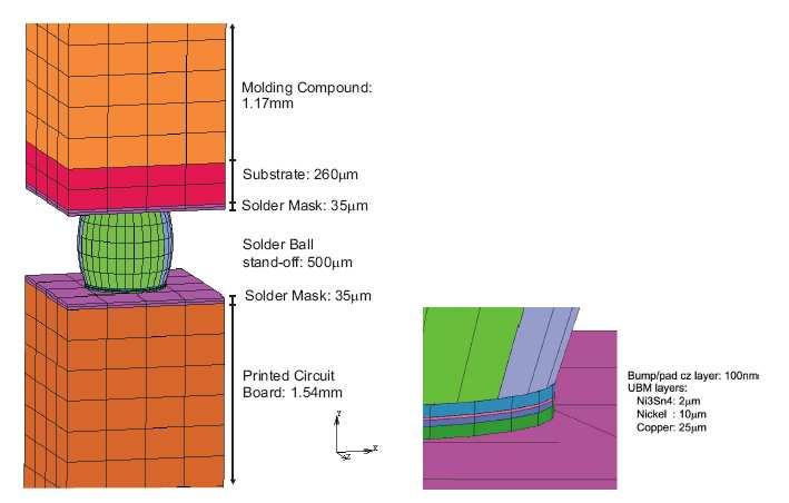
301 SOLDER JOINT FATIGUE