Graded Refractive-Index
|
|
|
- Γῆ Βλαστός
- 8 χρόνια πριν
- Προβολές:
Transcript
1 Graded Refractive-Index

2 Common Devices
3 Methodologies for Graded Refractive Index Methodologies: Ray Optics WKB Multilayer Modelling Solution requires: some knowledge of index profile n 2 x
4 Ray Optics for graded refractive index


5 Phase-change due to propagation k x T = tan 1 γ s k x + tan 1 γ c k x + m π k x x = ω c n x cos θ x = = ω c = ω c n 2 x n x sin θ x 2 = n 2 x N 2 k x x T N θ x i k x x i Δx i i n x i θ x i+1 n x i+1 ω c 0 x t n 2 x N 2 dx
6 Cladding-Film Interface k x T = tan 1 γ s k x + tan 1 γ c k x + m π N at x = 0 γ c = ω c N 2 n c 2 k x = ω c n 2 x = 0 N 2 = ω c n f 2 N 2 tan 1 γ c = tan 1 N2 2 n c π k x n 2 f N 2 2
7 Turning Point Interface k x T = tan 1 γ s k x + tan 1 γ c k x + m π N x t at x = x t k x = ω c n 2 x = x t + x N 2 γ s = ω c N 2 n 2 x = x t x n x = x t = N tan 1 γ c = tan 1 N 2 n 2 x=x t x tan 1 1 = π k x n 2 x=x t + x N 2 4
8 Bringing all the pieces together: k x T = tan 1 γ s k x + tan 1 γ c k x + m π ω c 0 x t n 2 x N 2 dx = π 4 + π 2 + m π x t N ω c 0 x t n 2 x N 2 dx = m π dispersion relation for a graded-refractive index waveguide
9 WKB Technique for graded refractive index

 (constant) (constant) When:")

10 Solving for TE modes d 2 E y x dx 2 + ω2 c 2 n2 x N 2 E y x = 0 k x x = ω c n 2 x N 2 If: n x = n f k x x = k x E y x = A e j k x x (constant) (constant) (constant) When: Δ n 2 x N 2 Δx/λ x 1 E y x = A x e j k x x x E y x = A x ej φ x where: k x x x φ x


11 Major steps in the derivation: E y x = A x ej φ x d 2 E y x dx 2 + ω2 c 2 n2 x N 2 E y x = 0 A A φ 2 = kx 2 A A + 2 j A φ + j A φ A φ 2 = kx 2 A 2 A φ + A φ = 0 A A φ 2 = kx 2 A A = φ 2 kx 2 A φ 2 kx 2 0 φ x = ± k x x dx 2 A φ + A φ = 0 A 2 φ = 0 A x = constant k x x
12 General Solution E y x = c 1 k x x e+j k x x dx + c 2 k x x e j k x x dx k x x = ω c n 2 x N 2

13 Cladding Region E y x = c 1 k x x e+j k x x dx + c 2 k x x e j k x x dx x k x x = ω c n 2 x N 2 for x < 0 k x x = ω c n 2 x N 2 = ω c n c 2 N 2 = j ω c N 2 n c 2 = j γc E y x = c 1 j γ c e 0 x γ c dx + c 2 j γ c e + 0 x γ c dx E y x = A γ c e γ c x
14 Guiding Region E y x = c 1 k x x e+j k x x dx + c 2 k x x e j k x x dx k x x = ω c n 2 x N 2 x for 0 < x < x t k x x = ω c n 2 x N 2 E y x = B k x x e+j x t x k x x dx + C k x x e j x t x k x x dx

15 Beyond Turning Point E y x = c 1 k x x e+j k x x dx + c 2 k x x e j k x x dx k x x = ω c n 2 x N 2 x for x > x t k x x = ω c n 2 x N 2 = j ω c N 2 n 2 x = j γ s x E y x = D γ s x e x x t γ s x dx

16 3D Waveguides Channel Waveguides Optical Fibers

 >")
17 Channel Waveguides x x y III T n 5 V I n 1 II n 3 n 2 IV n 4 y W typically: width(w) > thickness (T)

18 a) Marcatili s Method H y TM-like modes: H y & E x E x

19 Transverse confinement along x-axis, tangential H y Region I: H y x, y = H 1 cos k x x + φ 1 T < x < 0 Region II : x < T H y x, y = H 2 e γ x,2 x+t Region III: x > 0 H y x, y = H 3 e γ x,3 x k x T = tan 1 γ x,2 n 2 2 n 1 2 k x + tan 1 γ x,3 n 3 2 n 1 2 k x + p π
20 Lateral confinement along y-axis, tangential E x Region I: E x x, y = E 1 cos k y y + φ 2 W 2 < x < W 2 Region IV : E x x, y = E 4 e γ y,4 y W 2 y > W 2 Region V: E x x, y = E 5 e γ 5,y y+ W 2 y < W 2 k y W = tan 1 γ y,4 k y + tan 1 γ y,5 k y + q π
21 Finding the propagation constants: k x T = tan 1 γ 2 x,2 n 1 + tan 1 γ 2 x,3 n 1 n 2 2 k x n 2 3 k x + p π F 1 k x, γ x,2, γ x,3, β = 0 k y W = tan 1 γ y,4 k y + tan 1 γ y,5 k y + q π F 2 k y, γ x,4, γ x,5, β = 0 n 1 2 ω2 c 2 = k 1 2 = k x 2 + k y 2 + β 2 G 1 k x, k y, β = 0 n 2 2 ω2 c 2 = k 2 2 = γ x,2 2 + k y 2 + β 2 n 3 2 ω2 c 2 = k 3 2 = γ x,3 2 + k y 2 + β 2 n 4 2 ω2 c 2 = k 4 2 = k x 2 γ y,4 2 + β 2 n 5 2 ω2 c 2 = k 5 2 = k x 2 γ y,5 2 + β 2 G 2 γ x,2, k y, β = 0 G 3 γ x,3, k y, β = 0 G 4 k x, γ y,4, β = 0 G 5 k x, γ y,5, β = 0
22 b) Effective Index Method n f n s n c n f n s n s N I n s
23 TM-like modes I) n c, n f, T, n s (TM) F a M, b M N I, V I = 0 N I II) n s, N I, W, n s (TE) F a E, b E N II, V II = 0 N II
24 Criteria for Single-Mode Operation n f = n s + n with n n s Transverse confinement: I) Transverse confinement: cut-off condition for mode p : b I,p = 0 V I,p = tan 1 a I + p π Requirement for existence of only one mode in transverse direction: tan 1 a I < V I < tan 1 a I + π
25 Lateral confinement: II) Lateral confinement: cut-off condition for mode q : b II,q = 0 V II,q = tan 1 a II + q π it is a symmetric waveguide, so we have: a II = 0 Requirement for existence of only one mode in lateral direction: 0 < V II < π


26 A little bit of algebra leads to: V I = ω c T n f 2 n s 2 b I N I 2 n s 2 n f 2 n s 2 V II = ω c W N I 2 n s 2 = ω c W b I n f 2 n s 2 = W T V I b I 0 < V II < π 0 < W T < π V I b I and tan 1 a I < V I < tan 1 a I + π single-mode region a I


27 step-index multimode step-index singlemode GRIN Optical Fibers a cylindrical dielectric waveguide
28 Modes in Optical Fibers Cartesian coordinates 2 E x, y x E x, y y 2 + n2 ω 2 c 2 β2 E x, y = 0 E x, y, z, t = E x, y ej ω t β z Cylindrical coordinates 2 E r, φ r r E r, φ r + 1 r 2 2 E r, φ φ 2 + n2 ω 2 c 2 β2 E r, φ = 0 E r, φ, z, t = E r, φ ej ω t β z
29 Solutions E r, φ = u r e j l φ e d 2 u dr du r dr + n2 ω 2 c 2 β2 l2 r 2 u = 0 k T 2 n co 2 ω 2 c 2 β 2 γ 2 β 2 n cl 2 ω 2 c 2 Boundary conditions for E z, H z, E φ, H φ
30 Graphical Representation

31 Power Confinement Fraction of the power propagating inside the core against the V-number. Right above the cut-off, very little power is inside the core. As the core diameter increases, the power of the mode becomes confined inside the core.
32 Optical Attenuation 0.16 db = (3.6 %) 1 db = 10 log T


33 Numerical Aperture NA = n 0 sin θ 0 = n co 2 n cl 2 V-number V = 2π a λ n co 2 n cl 2 = 2π a λ NA single-mode operation V < Number of Guided Modes in an Optical Fiber M = 4 π 2 V2
34 Coupled Mode Theory

35 A few examples:
36 Decomposition into the eigenmodes of the original structure E t x, y, z = a α z α E t,α x, y e j β α z + radiation modes H t x, y, z = a α z α H t,α x, y e j β α z + radiation modes


37 After a Careful (& Long) Analysis, Final Result: ± da μ dz = j α a α z e j β α β μ z Κ μ,α Κ μ,α Κ t μ,α + Κz μ,α 4 Κ t μ,α ω ε x, y, z E t,μ Et,α dx dy 4Κ z μ,α ω ε ε ε + ε E z,μ E z,α dx dy whenever ε is a real number, then Κ μ,α = Κ α,μ


38 Co-Directional Couplers: A z 2 = cos 2 β c z + 2 β 2 sin2 β c z = c 1 F sin 2 β c z B z 2 Κ 2 = = β 2 sin2 β c z c F sin 2 β c z F Κ2 β 2 = Κ 2 c Κ A z 2 when: β b = β a β b β a 2 = 0 F = 1 β c Κ = Κ L = π 2 β c = π 2 Κ π 2 F = 0.2 F = 0.8 B z 2 z βc z βc


39 Counter-Directional Couplers = 0 Κ c = 0.2 A z 2 L = 5 A z 2 = 1 + F sinh2 α z L 1 + F sinh 2 α L B z 2 B z 2 = F sinh2 α z L 1 + F sinh 2 α L A z 2 L = 9 F Κ c 2 Κ c 2 2 > 1 when: = 0 L π Κ c B z 2
Homework 8 Model Solution Section
 MATH 004 Homework Solution Homework 8 Model Solution Section 14.5 14.6. 14.5. Use the Chain Rule to find dz where z cosx + 4y), x 5t 4, y 1 t. dz dx + dy y sinx + 4y)0t + 4) sinx + 4y) 1t ) 0t + 4t ) sinx
ECE Spring Prof. David R. Jackson ECE Dept. Notes 2
 ECE 634 Spring 6 Prof. David R. Jackson ECE Dept. Notes Fields in a Source-Free Region Example: Radiation from an aperture y PEC E t x Aperture Assume the following choice of vector potentials: A F = =
Areas and Lengths in Polar Coordinates
 Kiryl Tsishchanka Areas and Lengths in Polar Coordinates In this section we develop the formula for the area of a region whose boundary is given by a polar equation. We need to use the formula for the
Areas and Lengths in Polar Coordinates
 Kiryl Tsishchanka Areas and Lengths in Polar Coordinates In this section we develop the formula for the area of a region whose boundary is given by a polar equation. We need to use the formula for the
b. Use the parametrization from (a) to compute the area of S a as S a ds. Be sure to substitute for ds!
 to compute the area of S a as S a ds. Be sure to substitute for ds!") MTH U341 urface Integrals, tokes theorem, the divergence theorem To be turned in Wed., Dec. 1. 1. Let be the sphere of radius a, x 2 + y 2 + z 2 a 2. a. Use spherical coordinates (with ρ a) to parametrize.
MTH U341 urface Integrals, tokes theorem, the divergence theorem To be turned in Wed., Dec. 1. 1. Let be the sphere of radius a, x 2 + y 2 + z 2 a 2. a. Use spherical coordinates (with ρ a) to parametrize.
Inverse trigonometric functions & General Solution of Trigonometric Equations. ------------------ ----------------------------- -----------------
 Inverse trigonometric functions & General Solution of Trigonometric Equations. 1. Sin ( ) = a) b) c) d) Ans b. Solution : Method 1. Ans a: 17 > 1 a) is rejected. w.k.t Sin ( sin ) = d is rejected. If sin
Appendix A. Curvilinear coordinates. A.1 Lamé coefficients. Consider set of equations. ξ i = ξ i (x 1,x 2,x 3 ), i = 1,2,3
, i = 1,2,3") Appendix A Curvilinear coordinates A. Lamé coefficients Consider set of equations ξ i = ξ i x,x 2,x 3, i =,2,3 where ξ,ξ 2,ξ 3 independent, single-valued and continuous x,x 2,x 3 : coordinates of point
Appendix A Curvilinear coordinates A. Lamé coefficients Consider set of equations ξ i = ξ i x,x 2,x 3, i =,2,3 where ξ,ξ 2,ξ 3 independent, single-valued and continuous x,x 2,x 3 : coordinates of point
1 String with massive end-points
 1 String with massive end-points Πρόβλημα 5.11:Θεωρείστε μια χορδή μήκους, τάσης T, με δύο σημειακά σωματίδια στα άκρα της, το ένα μάζας m, και το άλλο μάζας m. α) Μελετώντας την κίνηση των άκρων βρείτε
D Alembert s Solution to the Wave Equation
 D Alembert s Solution to the Wave Equation MATH 467 Partial Differential Equations J. Robert Buchanan Department of Mathematics Fall 2018 Objectives In this lesson we will learn: a change of variable technique
Second Order RLC Filters
 ECEN 60 Circuits/Electronics Spring 007-0-07 P. Mathys Second Order RLC Filters RLC Lowpass Filter A passive RLC lowpass filter (LPF) circuit is shown in the following schematic. R L C v O (t) Using phasor
Integrals in cylindrical, spherical coordinates (Sect. 15.7)
") Integrals in clindrical, spherical coordinates (Sect. 5.7 Integration in spherical coordinates. Review: Clindrical coordinates. Spherical coordinates in space. Triple integral in spherical coordinates.
Integrals in clindrical, spherical coordinates (Sect. 5.7 Integration in spherical coordinates. Review: Clindrical coordinates. Spherical coordinates in space. Triple integral in spherical coordinates.
9.09. # 1. Area inside the oval limaçon r = cos θ. To graph, start with θ = 0 so r = 6. Compute dr
 9.9 #. Area inside the oval limaçon r = + cos. To graph, start with = so r =. Compute d = sin. Interesting points are where d vanishes, or at =,,, etc. For these values of we compute r:,,, and the values
Spherical Coordinates
 Spherical Coordinates MATH 311, Calculus III J. Robert Buchanan Department of Mathematics Fall 2011 Spherical Coordinates Another means of locating points in three-dimensional space is known as the spherical
What happens when two or more waves overlap in a certain region of space at the same time?
 Wave Superposition What happens when two or more waves overlap in a certain region of space at the same time? To find the resulting wave according to the principle of superposition we should sum the fields
Answer sheet: Third Midterm for Math 2339
 Answer sheet: Third Midterm for Math 339 November 3, Problem. Calculate the iterated integrals (Simplify as much as possible) (a) e sin(x) dydx y e sin(x) dydx y sin(x) ln y ( cos(x)) ye y dx sin(x)(lne
Dr. D. Dinev, Department of Structural Mechanics, UACEG
 Lecture 4 Material behavior: Constitutive equations Field of the game Print version Lecture on Theory of lasticity and Plasticity of Dr. D. Dinev, Department of Structural Mechanics, UACG 4.1 Contents
forms This gives Remark 1. How to remember the above formulas: Substituting these into the equation we obtain with
 Week 03: C lassification of S econd- Order L inear Equations In last week s lectures we have illustrated how to obtain the general solutions of first order PDEs using the method of characteristics. We
Solutions to Exercise Sheet 5
 Solutions to Eercise Sheet 5 jacques@ucsd.edu. Let X and Y be random variables with joint pdf f(, y) = 3y( + y) where and y. Determine each of the following probabilities. Solutions. a. P (X ). b. P (X
Phys460.nb Solution for the t-dependent Schrodinger s equation How did we find the solution? (not required)
") Phys460.nb 81 ψ n (t) is still the (same) eigenstate of H But for tdependent H. The answer is NO. 5.5.5. Solution for the tdependent Schrodinger s equation If we assume that at time t 0, the electron starts
Phys460.nb 81 ψ n (t) is still the (same) eigenstate of H But for tdependent H. The answer is NO. 5.5.5. Solution for the tdependent Schrodinger s equation If we assume that at time t 0, the electron starts
Lifting Entry (continued)
") ifting Entry (continued) Basic planar dynamics of motion, again Yet another equilibrium glide Hypersonic phugoid motion Planar state equations MARYAN 1 01 avid. Akin - All rights reserved http://spacecraft.ssl.umd.edu
ifting Entry (continued) Basic planar dynamics of motion, again Yet another equilibrium glide Hypersonic phugoid motion Planar state equations MARYAN 1 01 avid. Akin - All rights reserved http://spacecraft.ssl.umd.edu
Differential equations
 Differential equations Differential equations: An equation inoling one dependent ariable and its deriaties w. r. t one or more independent ariables is called a differential equation. Order of differential
Note: Please use the actual date you accessed this material in your citation.
 MIT OpenCourseWare http://ocw.mit.edu 6.03/ESD.03J Electromagnetics and Applications, Fall 005 Please use the following citation format: Markus Zahn, 6.03/ESD.03J Electromagnetics and Applications, Fall
A Determination Method of Diffusion-Parameter Values in the Ion-Exchange Optical Waveguides in Soda-Lime glass Made by Diluted AgNO 3 with NaNO 3
 大阪電気通信大学研究論集 ( 自然科学編 ) 第 51 号 A Determination Method of Diffusion-Parameter Values in the Ion-Exchange Optical Waveguides in Soda-Lime glass Made by Diluted AgNO 3 with NaNO 3 Takuya IWATA and Kiyoshi
Lecture 26: Circular domains
 Introductory lecture notes on Partial Differential Equations - c Anthony Peirce. Not to be copied, used, or revised without eplicit written permission from the copyright owner. 1 Lecture 6: Circular domains
Απόκριση σε Μοναδιαία Ωστική Δύναμη (Unit Impulse) Απόκριση σε Δυνάμεις Αυθαίρετα Μεταβαλλόμενες με το Χρόνο. Απόστολος Σ.
 Απόκριση σε Δυνάμεις Αυθαίρετα Μεταβαλλόμενες με το Χρόνο. Απόστολος Σ.") Απόκριση σε Δυνάμεις Αυθαίρετα Μεταβαλλόμενες με το Χρόνο The time integral of a force is referred to as impulse, is determined by and is obtained from: Newton s 2 nd Law of motion states that the action
Απόκριση σε Δυνάμεις Αυθαίρετα Μεταβαλλόμενες με το Χρόνο The time integral of a force is referred to as impulse, is determined by and is obtained from: Newton s 2 nd Law of motion states that the action
Matrices and Determinants
 Matrices and Determinants SUBJECTIVE PROBLEMS: Q 1. For what value of k do the following system of equations possess a non-trivial (i.e., not all zero) solution over the set of rationals Q? x + ky + 3z
Lecture 2: Dirac notation and a review of linear algebra Read Sakurai chapter 1, Baym chatper 3
 Lecture 2: Dirac notation and a review of linear algebra Read Sakurai chapter 1, Baym chatper 3 1 State vector space and the dual space Space of wavefunctions The space of wavefunctions is the set of all
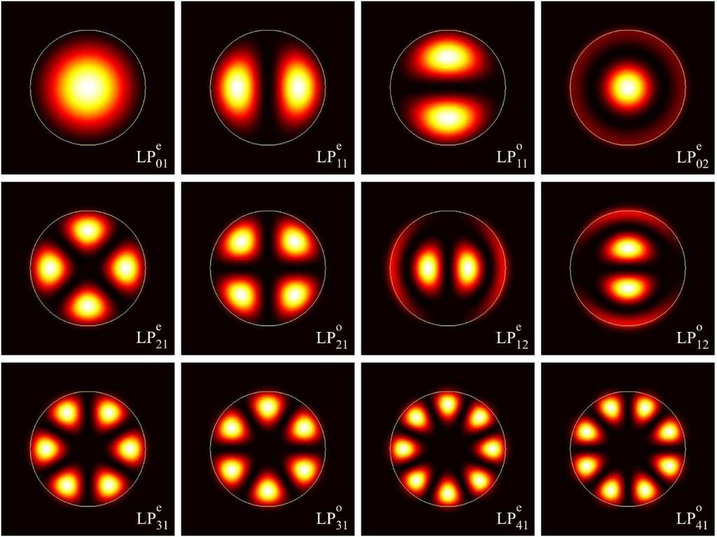
ΟΛΟΚΛΗΡΩΜΕΝΗ ΟΠΤΙΚΗ. Χειμερινό Εξάμηνο Γενικές Πληροφορίες. Αιθ. 008(Ν. Κτίρια, ΗΜΜΥ) Ηλίας Ν. Γλύτσης (Παλαιά Κτίρια ΗΜΜΥ)
 Ηλίας Ν. Γλύτσης (Παλαιά Κτίρια ΗΜΜΥ)") 04/10/2017 ΟΛΟΚΛΗΡΩΜΕΝΗ ΟΠΤΙΚΗ Χειμερινό Εξάμηνο 2017-2018 Γενικές Πληροφορίες Ώρα: Τετάρτη 08:45-11:30 Αίθουσα: Αιθ. 008(Ν. Κτίρια, ΗΜΜΥ) Καθηγητής: Ηλίας Ν. Γλύτσης Γραφείο: 2.2.22 (Παλαιά Κτίρια ΗΜΜΥ)
04/10/2017 ΟΛΟΚΛΗΡΩΜΕΝΗ ΟΠΤΙΚΗ Χειμερινό Εξάμηνο 2017-2018 Γενικές Πληροφορίες Ώρα: Τετάρτη 08:45-11:30 Αίθουσα: Αιθ. 008(Ν. Κτίρια, ΗΜΜΥ) Καθηγητής: Ηλίας Ν. Γλύτσης Γραφείο: 2.2.22 (Παλαιά Κτίρια ΗΜΜΥ)
Variational Wavefunction for the Helium Atom
 Technische Universität Graz Institut für Festkörperphysik Student project Variational Wavefunction for the Helium Atom Molecular and Solid State Physics 53. submitted on: 3. November 9 by: Markus Krammer
Differentiation exercise show differential equation
 Differentiation exercise show differential equation 1. If y x sin 2x, prove that x d2 y 2 2 + 2y x + 4xy 0 y x sin 2x sin 2x + 2x cos 2x 2 2cos 2x + (2 cos 2x 4x sin 2x) x d2 y 2 2 + 2y x + 4xy (2x cos
ANSWERSHEET (TOPIC = DIFFERENTIAL CALCULUS) COLLECTION #2. h 0 h h 0 h h 0 ( ) g k = g 0 + g 1 + g g 2009 =?
 COLLECTION #2. h 0 h h 0 h h 0 ( ) g k = g 0 + g 1 + g g 2009 =?") Teko Classes IITJEE/AIEEE Maths by SUHAAG SIR, Bhopal, Ph (0755) 3 00 000 www.tekoclasses.com ANSWERSHEET (TOPIC DIFFERENTIAL CALCULUS) COLLECTION # Question Type A.Single Correct Type Q. (A) Sol least
Teko Classes IITJEE/AIEEE Maths by SUHAAG SIR, Bhopal, Ph (0755) 3 00 000 www.tekoclasses.com ANSWERSHEET (TOPIC DIFFERENTIAL CALCULUS) COLLECTION # Question Type A.Single Correct Type Q. (A) Sol least
Numerical Analysis FMN011
 Numerical Analysis FMN011 Carmen Arévalo Lund University carmen@maths.lth.se Lecture 12 Periodic data A function g has period P if g(x + P ) = g(x) Model: Trigonometric polynomial of order M T M (x) =
Example Sheet 3 Solutions
 Example Sheet 3 Solutions. i Regular Sturm-Liouville. ii Singular Sturm-Liouville mixed boundary conditions. iii Not Sturm-Liouville ODE is not in Sturm-Liouville form. iv Regular Sturm-Liouville note
derivation of the Laplacian from rectangular to spherical coordinates
 derivation of the Laplacian from rectangular to spherical coordinates swapnizzle 03-03- :5:43 We begin by recognizing the familiar conversion from rectangular to spherical coordinates (note that φ is used
Appendix to On the stability of a compressible axisymmetric rotating flow in a pipe. By Z. Rusak & J. H. Lee
 Appendi to On the stability of a compressible aisymmetric rotating flow in a pipe By Z. Rusak & J. H. Lee Journal of Fluid Mechanics, vol. 5 4, pp. 5 4 This material has not been copy-edited or typeset
SOLUTIONS TO MATH38181 EXTREME VALUES AND FINANCIAL RISK EXAM
 SOLUTIONS TO MATH38181 EXTREME VALUES AND FINANCIAL RISK EXAM Solutions to Question 1 a) The cumulative distribution function of T conditional on N n is Pr T t N n) Pr max X 1,..., X N ) t N n) Pr max
6.4 Superposition of Linear Plane Progressive Waves
 .0 - Marine Hydrodynamics, Spring 005 Lecture.0 - Marine Hydrodynamics Lecture 6.4 Superposition of Linear Plane Progressive Waves. Oblique Plane Waves z v k k k z v k = ( k, k z ) θ (Looking up the y-ais
Mock Exam 7. 1 Hong Kong Educational Publishing Company. Section A 1. Reference: HKDSE Math M Q2 (a) (1 + kx) n 1M + 1A = (1) =
 (1 + kx) n 1M + 1A = (1) =") Mock Eam 7 Mock Eam 7 Section A. Reference: HKDSE Math M 0 Q (a) ( + k) n nn ( )( k) + nk ( ) + + nn ( ) k + nk + + + A nk... () nn ( ) k... () From (), k...() n Substituting () into (), nn ( ) n 76n 76n
Mock Eam 7 Mock Eam 7 Section A. Reference: HKDSE Math M 0 Q (a) ( + k) n nn ( )( k) + nk ( ) + + nn ( ) k + nk + + + A nk... () nn ( ) k... () From (), k...() n Substituting () into (), nn ( ) n 76n 76n
Partial Differential Equations in Biology The boundary element method. March 26, 2013
 The boundary element method March 26, 203 Introduction and notation The problem: u = f in D R d u = ϕ in Γ D u n = g on Γ N, where D = Γ D Γ N, Γ D Γ N = (possibly, Γ D = [Neumann problem] or Γ N = [Dirichlet
Radiation Stress Concerned with the force (or momentum flux) exerted on the right hand side of a plane by water on the left hand side of the plane.
 exerted on the right hand side of a plane by water on the left hand side of the plane.") upplement on Radiation tress and Wave etup/et down Radiation tress oncerned wit te force (or momentum flu) eerted on te rit and side of a plane water on te left and side of te plane. plane z "Radiation
upplement on Radiation tress and Wave etup/et down Radiation tress oncerned wit te force (or momentum flu) eerted on te rit and side of a plane water on te left and side of te plane. plane z "Radiation
ES440/ES911: CFD. Chapter 5. Solution of Linear Equation Systems
 ES440/ES911: CFD Chapter 5. Solution of Linear Equation Systems Dr Yongmann M. Chung http://www.eng.warwick.ac.uk/staff/ymc/es440.html Y.M.Chung@warwick.ac.uk School of Engineering & Centre for Scientific
Strain gauge and rosettes
 Strain gauge and rosettes Introduction A strain gauge is a device which is used to measure strain (deformation) on an object subjected to forces. Strain can be measured using various types of devices classified
Problem Set 9 Solutions. θ + 1. θ 2 + cotθ ( ) sinθ e iφ is an eigenfunction of the ˆ L 2 operator. / θ 2. φ 2. sin 2 θ φ 2. ( ) = e iφ. = e iφ cosθ.
 sinθ e iφ is an eigenfunction of the ˆ L 2 operator. / θ 2. φ 2. sin 2 θ φ 2. ( ) = e iφ. = e iφ cosθ.") Chemistry 362 Dr Jean M Standard Problem Set 9 Solutions The ˆ L 2 operator is defined as Verify that the angular wavefunction Y θ,φ) Also verify that the eigenvalue is given by 2! 2 & L ˆ 2! 2 2 θ 2 +
Chemistry 362 Dr Jean M Standard Problem Set 9 Solutions The ˆ L 2 operator is defined as Verify that the angular wavefunction Y θ,φ) Also verify that the eigenvalue is given by 2! 2 & L ˆ 2! 2 2 θ 2 +
Section 8.3 Trigonometric Equations
 99 Section 8. Trigonometric Equations Objective 1: Solve Equations Involving One Trigonometric Function. In this section and the next, we will exple how to solving equations involving trigonometric functions.
PARTIAL NOTES for 6.1 Trigonometric Identities
 PARTIAL NOTES for 6.1 Trigonometric Identities tanθ = sinθ cosθ cotθ = cosθ sinθ BASIC IDENTITIES cscθ = 1 sinθ secθ = 1 cosθ cotθ = 1 tanθ PYTHAGOREAN IDENTITIES sin θ + cos θ =1 tan θ +1= sec θ 1 + cot
Higher Derivative Gravity Theories
 Higher Derivative Gravity Theories Black Holes in AdS space-times James Mashiyane Supervisor: Prof Kevin Goldstein University of the Witwatersrand Second Mandelstam, 20 January 2018 James Mashiyane WITS)
Jackson 2.25 Homework Problem Solution Dr. Christopher S. Baird University of Massachusetts Lowell
 Jackson 2.25 Hoework Proble Solution Dr. Christopher S. Baird University of Massachusetts Lowell PROBLEM: Two conducting planes at zero potential eet along the z axis, aking an angle β between the, as
10/3/ revolution = 360 = 2 π radians = = x. 2π = x = 360 = : Measures of Angles and Rotations
 //.: Measures of Angles and Rotations I. Vocabulary A A. Angle the union of two rays with a common endpoint B. BA and BC C. B is the vertex. B C D. You can think of BA as the rotation of (clockwise) with
Second Order Partial Differential Equations
 Chapter 7 Second Order Partial Differential Equations 7.1 Introduction A second order linear PDE in two independent variables (x, y Ω can be written as A(x, y u x + B(x, y u xy + C(x, y u u u + D(x, y
Approximation of distance between locations on earth given by latitude and longitude
 Approximation of distance between locations on earth given by latitude and longitude Jan Behrens 2012-12-31 In this paper we shall provide a method to approximate distances between two points on earth
Calculating the propagation delay of coaxial cable
 Your source for quality GNSS Networking Solutions and Design Services! Page 1 of 5 Calculating the propagation delay of coaxial cable The delay of a cable or velocity factor is determined by the dielectric
Lifting Entry 2. Basic planar dynamics of motion, again Yet another equilibrium glide Hypersonic phugoid motion MARYLAND U N I V E R S I T Y O F
 ifting Entry Basic planar dynamics of motion, again Yet another equilibrium glide Hypersonic phugoid motion MARYAN 1 010 avid. Akin - All rights reserved http://spacecraft.ssl.umd.edu ifting Atmospheric
1. (a) (5 points) Find the unit tangent and unit normal vectors T and N to the curve. r(t) = 3cost, 4t, 3sint
 (5 points) Find the unit tangent and unit normal vectors T and N to the curve. r(t) = 3cost, 4t, 3sint") 1. a) 5 points) Find the unit tangent and unit normal vectors T and N to the curve at the point P, π, rt) cost, t, sint ). b) 5 points) Find curvature of the curve at the point P. Solution: a) r t) sint,,
1. a) 5 points) Find the unit tangent and unit normal vectors T and N to the curve at the point P, π, rt) cost, t, sint ). b) 5 points) Find curvature of the curve at the point P. Solution: a) r t) sint,,
Chapter 6: Systems of Linear Differential. be continuous functions on the interval
 Chapter 6: Systems of Linear Differential Equations Let a (t), a 2 (t),..., a nn (t), b (t), b 2 (t),..., b n (t) be continuous functions on the interval I. The system of n first-order differential equations
Section 8.2 Graphs of Polar Equations
 Section 8. Graphs of Polar Equations Graphing Polar Equations The graph of a polar equation r = f(θ), or more generally F(r,θ) = 0, consists of all points P that have at least one polar representation
Block Ciphers Modes. Ramki Thurimella
 Block Ciphers Modes Ramki Thurimella Only Encryption I.e. messages could be modified Should not assume that nonsensical messages do no harm Always must be combined with authentication 2 Padding Must be
CHAPTER (2) Electric Charges, Electric Charge Densities and Electric Field Intensity
 Electric Charges, Electric Charge Densities and Electric Field Intensity") CHAPTE () Electric Chrges, Electric Chrge Densities nd Electric Field Intensity Chrge Configurtion ) Point Chrge: The concept of the point chrge is used when the dimensions of n electric chrge distriution
CHAPTE () Electric Chrges, Electric Chrge Densities nd Electric Field Intensity Chrge Configurtion ) Point Chrge: The concept of the point chrge is used when the dimensions of n electric chrge distriution
Other Test Constructions: Likelihood Ratio & Bayes Tests
 Other Test Constructions: Likelihood Ratio & Bayes Tests Side-Note: So far we have seen a few approaches for creating tests such as Neyman-Pearson Lemma ( most powerful tests of H 0 : θ = θ 0 vs H 1 :
Laplace s Equation in Spherical Polar Coördinates
 Laplace s Equation in Spheical Pola Coödinates C. W. David Dated: Januay 3, 001 We stat with the pimitive definitions I. x = sin θ cos φ y = sin θ sin φ z = cos θ thei inveses = x y z θ = cos 1 z = z cos1
ECE 468: Digital Image Processing. Lecture 8
 ECE 468: Digital Image Processing Lecture 8 Prof. Sinisa Todorovic sinisa@eecs.oregonstate.edu 1 Image Reconstruction from Projections X-ray computed tomography: X-raying an object from different directions
EE512: Error Control Coding
 EE512: Error Control Coding Solution for Assignment on Finite Fields February 16, 2007 1. (a) Addition and Multiplication tables for GF (5) and GF (7) are shown in Tables 1 and 2. + 0 1 2 3 4 0 0 1 2 3
DETERMINATION OF DYNAMIC CHARACTERISTICS OF A 2DOF SYSTEM. by Zoran VARGA, Ms.C.E.
 DETERMINATION OF DYNAMIC CHARACTERISTICS OF A 2DOF SYSTEM by Zoran VARGA, Ms.C.E. Euro-Apex B.V. 1990-2012 All Rights Reserved. The 2 DOF System Symbols m 1 =3m [kg] m 2 =8m m=10 [kg] l=2 [m] E=210000
C.S. 430 Assignment 6, Sample Solutions
 C.S. 430 Assignment 6, Sample Solutions Paul Liu November 15, 2007 Note that these are sample solutions only; in many cases there were many acceptable answers. 1 Reynolds Problem 10.1 1.1 Normal-order
Fourier Series. MATH 211, Calculus II. J. Robert Buchanan. Spring Department of Mathematics
 Fourier Series MATH 211, Calculus II J. Robert Buchanan Department of Mathematics Spring 2018 Introduction Not all functions can be represented by Taylor series. f (k) (c) A Taylor series f (x) = (x c)
Orbital angular momentum and the spherical harmonics
 Orbital angular momentum and the spherical harmonics March 8, 03 Orbital angular momentum We compare our result on representations of rotations with our previous experience of angular momentum, defined
Econ 2110: Fall 2008 Suggested Solutions to Problem Set 8 questions or comments to Dan Fetter 1
 Eon : Fall 8 Suggested Solutions to Problem Set 8 Email questions or omments to Dan Fetter Problem. Let X be a salar with density f(x, θ) (θx + θ) [ x ] with θ. (a) Find the most powerful level α test
Oscillatory Gap Damping
 Oscillatory Gap Damping Find the damping due to the linear motion of a viscous gas in in a gap with an oscillating size: ) Find the motion in a gap due to an oscillating external force; ) Recast the solution
SOLUTIONS TO MATH38181 EXTREME VALUES AND FINANCIAL RISK EXAM
 SOLUTIONS TO MATH38181 EXTREME VALUES AND FINANCIAL RISK EXAM Solutions to Question 1 a) The cumulative distribution function of T conditional on N n is Pr (T t N n) Pr (max (X 1,..., X N ) t N n) Pr (max
wave energy Superposition of linear plane progressive waves Marine Hydrodynamics Lecture Oblique Plane Waves:
 3.0 Marine Hydrodynamics, Fall 004 Lecture 0 Copyriht c 004 MIT - Department of Ocean Enineerin, All rihts reserved. 3.0 - Marine Hydrodynamics Lecture 0 Free-surface waves: wave enery linear superposition,
Pg The perimeter is P = 3x The area of a triangle is. where b is the base, h is the height. In our case b = x, then the area is
 Pg. 9. The perimeter is P = The area of a triangle is A = bh where b is the base, h is the height 0 h= btan 60 = b = b In our case b =, then the area is A = = 0. By Pythagorean theorem a + a = d a a =
 y(t) S x(t) S dy dx E, E E T1 T2 T1 T2 1 T 1 T 2 2 T 2 1 T 2 2 3 T 3 1 T 3 2... V o R R R T V CC P F A P g h V ext V sin 2 S f S t V 1 V 2 V out sin 2 f S t x 1 F k q K x q K k F d F x d V
Problem 3.16 Given B = ˆx(z 3y) +ŷ(2x 3z) ẑ(x+y), find a unit vector parallel. Solution: At P = (1,0, 1), ˆb = B
 +ŷ(2x 3z) ẑ(x+y), find a unit vector parallel. Solution: At P = (1,0, 1), ˆb = B") Problem 3.6 Given B = ˆxz 3y) +ŷx 3z) ẑx+y), find a unit vector parallel to B at point P =,0, ). Solution: At P =,0, ), B = ˆx )+ŷ+3) ẑ) = ˆx+ŷ5 ẑ, ˆb = B B = ˆx+ŷ5 ẑ = ˆx+ŷ5 ẑ. +5+ 7 Problem 3.4 Convert
Problem 3.6 Given B = ˆxz 3y) +ŷx 3z) ẑx+y), find a unit vector parallel to B at point P =,0, ). Solution: At P =,0, ), B = ˆx )+ŷ+3) ẑ) = ˆx+ŷ5 ẑ, ˆb = B B = ˆx+ŷ5 ẑ = ˆx+ŷ5 ẑ. +5+ 7 Problem 3.4 Convert
Statistical Inference I Locally most powerful tests
 Statistical Inference I Locally most powerful tests Shirsendu Mukherjee Department of Statistics, Asutosh College, Kolkata, India. shirsendu st@yahoo.co.in So far we have treated the testing of one-sided
Geodesic Equations for the Wormhole Metric
 Geodesic Equations for the Wormhole Metric Dr R Herman Physics & Physical Oceanography, UNCW February 14, 2018 The Wormhole Metric Morris and Thorne wormhole metric: [M S Morris, K S Thorne, Wormholes
The Simply Typed Lambda Calculus
 Type Inference Instead of writing type annotations, can we use an algorithm to infer what the type annotations should be? That depends on the type system. For simple type systems the answer is yes, and
3.5 - Boundary Conditions for Potential Flow
 13.021 Marine Hydrodynamics, Fall 2004 Lecture 10 Copyright c 2004 MIT - Department of Ocean Engineering, All rights reserved. 13.021 - Marine Hydrodynamics Lecture 10 3.5 - Boundary Conditions for Potential
Practice Exam 2. Conceptual Questions. 1. State a Basic identity and then verify it. (a) Identity: Solution: One identity is csc(θ) = 1
 Identity: Solution: One identity is csc(θ) = 1") Conceptual Questions. State a Basic identity and then verify it. a) Identity: Solution: One identity is cscθ) = sinθ) Practice Exam b) Verification: Solution: Given the point of intersection x, y) of the
Conceptual Questions. State a Basic identity and then verify it. a) Identity: Solution: One identity is cscθ) = sinθ) Practice Exam b) Verification: Solution: Given the point of intersection x, y) of the
Answers - Worksheet A ALGEBRA PMT. 1 a = 7 b = 11 c = 1 3. e = 0.1 f = 0.3 g = 2 h = 10 i = 3 j = d = k = 3 1. = 1 or 0.5 l =
 C ALGEBRA Answers - Worksheet A a 7 b c d e 0. f 0. g h 0 i j k 6 8 or 0. l or 8 a 7 b 0 c 7 d 6 e f g 6 h 8 8 i 6 j k 6 l a 9 b c d 9 7 e 00 0 f 8 9 a b 7 7 c 6 d 9 e 6 6 f 6 8 g 9 h 0 0 i j 6 7 7 k 9
Homework 3 Solutions
 Homework 3 Solutions Igor Yanovsky (Math 151A TA) Problem 1: Compute the absolute error and relative error in approximations of p by p. (Use calculator!) a) p π, p 22/7; b) p π, p 3.141. Solution: For
( y) Partial Differential Equations
 Partial Differential Equations") Partial Dierential Equations Linear P.D.Es. contains no owers roducts o the deendent variables / an o its derivatives can occasionall be solved. Consider eamle ( ) a (sometimes written as a ) we can integrate
Partial Dierential Equations Linear P.D.Es. contains no owers roducts o the deendent variables / an o its derivatives can occasionall be solved. Consider eamle ( ) a (sometimes written as a ) we can integrate
Rectangular Polar Parametric
 Harold s Precalculus Rectangular Polar Parametric Cheat Sheet 15 October 2017 Point Line Rectangular Polar Parametric f(x) = y (x, y) (a, b) Slope-Intercept Form: y = mx + b Point-Slope Form: y y 0 = m
Exercises 10. Find a fundamental matrix of the given system of equations. Also find the fundamental matrix Φ(t) satisfying Φ(0) = I. 1.
 satisfying Φ(0) = I. 1.") Exercises 0 More exercises are available in Elementary Differential Equations. If you have a problem to solve any of them, feel free to come to office hour. Problem Find a fundamental matrix of the given
Exercises 0 More exercises are available in Elementary Differential Equations. If you have a problem to solve any of them, feel free to come to office hour. Problem Find a fundamental matrix of the given
38 Te(OH) 6 2NH 4 H 2 PO 4 (NH 4 ) 2 HPO 4
 6 2NH 4 H 2 PO 4 (NH 4 ) 2 HPO 4") Fig. A-1-1. Te(OH) NH H PO (NH ) HPO (TAAP). Projection of the crystal structure along the b direction [Ave]. 9 1. 7.5 ( a a )/ a [1 ] ( b b )/ b [1 ] 5..5 1.5 1 1.5 ( c c )/ c [1 ].5 1. 1.5. Angle β 1.
Fig. A-1-1. Te(OH) NH H PO (NH ) HPO (TAAP). Projection of the crystal structure along the b direction [Ave]. 9 1. 7.5 ( a a )/ a [1 ] ( b b )/ b [1 ] 5..5 1.5 1 1.5 ( c c )/ c [1 ].5 1. 1.5. Angle β 1.
Finite difference method for 2-D heat equation
 Finite difference method for 2-D heat equation Praveen. C praveen@math.tifrbng.res.in Tata Institute of Fundamental Research Center for Applicable Mathematics Bangalore 560065 http://math.tifrbng.res.in/~praveen
MathCity.org Merging man and maths
 MathCity.org Merging man and maths Exercise 10. (s) Page Textbook of Algebra and Trigonometry for Class XI Available online @, Version:.0 Question # 1 Find the values of sin, and tan when: 1 π (i) (ii)
CHAPTER 25 SOLVING EQUATIONS BY ITERATIVE METHODS
 CHAPTER 5 SOLVING EQUATIONS BY ITERATIVE METHODS EXERCISE 104 Page 8 1. Find the positive root of the equation x + 3x 5 = 0, correct to 3 significant figures, using the method of bisection. Let f(x) =
Space-Time Symmetries
 Chapter Space-Time Symmetries In classical fiel theory any continuous symmetry of the action generates a conserve current by Noether's proceure. If the Lagrangian is not invariant but only shifts by a
Section 7.6 Double and Half Angle Formulas
 09 Section 7. Double and Half Angle Fmulas To derive the double-angles fmulas, we will use the sum of two angles fmulas that we developed in the last section. We will let α θ and β θ: cos(θ) cos(θ + θ)
Durbin-Levinson recursive method
 Durbin-Levinson recursive method A recursive method for computing ϕ n is useful because it avoids inverting large matrices; when new data are acquired, one can update predictions, instead of starting again
Section 9.2 Polar Equations and Graphs
 180 Section 9. Polar Equations and Graphs In this section, we will be graphing polar equations on a polar grid. In the first few examples, we will write the polar equation in rectangular form to help identify
(As on April 16, 2002 no changes since Dec 24.)
") ~rprice/area51/documents/roswell.tex ROSWELL COORDINATES FOR TWO CENTERS As on April 16, 00 no changes since Dec 4. I. Definitions of coordinates We define the Roswell coordinates χ, Θ. A better name will
~rprice/area51/documents/roswell.tex ROSWELL COORDINATES FOR TWO CENTERS As on April 16, 00 no changes since Dec 4. I. Definitions of coordinates We define the Roswell coordinates χ, Θ. A better name will
Srednicki Chapter 55
 Srednicki Chapter 55 QFT Problems & Solutions A. George August 3, 03 Srednicki 55.. Use equations 55.3-55.0 and A i, A j ] = Π i, Π j ] = 0 (at equal times) to verify equations 55.-55.3. This is our third
26 28 Find an equation of the tangent line to the curve at the given point Discuss the curve under the guidelines of Section
 SECTION 5. THE NATURAL LOGARITHMIC FUNCTION 5. THE NATURAL LOGARITHMIC FUNCTION A Click here for answers. S Click here for solutions. 4 Use the Laws of Logarithms to epand the quantit.. ln ab. ln c. ln
F19MC2 Solutions 9 Complex Analysis
 F9MC Solutions 9 Complex Analysis. (i) Let f(z) = eaz +z. Then f is ifferentiable except at z = ±i an so by Cauchy s Resiue Theorem e az z = πi[res(f,i)+res(f, i)]. +z C(,) Since + has zeros of orer at
Symmetry. March 31, 2013
 Symmetry March 3, 203 The Lie Derivative With or without the covariant derivative, which requires a connection on all of spacetime, there is another sort of derivation called the Lie derivative, which
Magnetically Coupled Circuits
 DR. GYURCSEK ISTVÁN Magnetically Coupled Circuits Sources and additional materials (recommended) Dr. Gyurcsek Dr. Elmer: Theories in Electric Circuits, GlobeEdit, 2016, ISBN:978-3-330-71341-3 Ch. Alexander,
HOMEWORK 4 = G. In order to plot the stress versus the stretch we define a normalized stretch:
 HOMEWORK 4 Problem a For the fast loading case, we want to derive the relationship between P zz and λ z. We know that the nominal stress is expressed as: P zz = ψ λ z where λ z = λ λ z. Therefore, applying
Problem 3.1 Vector A starts at point (1, 1, 3) and ends at point (2, 1,0). Find a unit vector in the direction of A. Solution: A = 1+9 = 3.
 and ends at point (2, 1,0). Find a unit vector in the direction of A. Solution: A = 1+9 = 3.") Problem 3.1 Vector A starts at point (1, 1, 3) and ends at point (, 1,0). Find a unit vector in the direction of A. Solution: A = ˆx( 1)+ŷ( 1 ( 1))+ẑ(0 ( 3)) = ˆx+ẑ3, A = 1+9 = 3.16, â = A A = ˆx+ẑ3 3.16
Problem 3.1 Vector A starts at point (1, 1, 3) and ends at point (, 1,0). Find a unit vector in the direction of A. Solution: A = ˆx( 1)+ŷ( 1 ( 1))+ẑ(0 ( 3)) = ˆx+ẑ3, A = 1+9 = 3.16, â = A A = ˆx+ẑ3 3.16
CRASH COURSE IN PRECALCULUS
 CRASH COURSE IN PRECALCULUS Shiah-Sen Wang The graphs are prepared by Chien-Lun Lai Based on : Precalculus: Mathematics for Calculus by J. Stuwart, L. Redin & S. Watson, 6th edition, 01, Brooks/Cole Chapter
Overview. Transition Semantics. Configurations and the transition relation. Executions and computation
 Overview Transition Semantics Configurations and the transition relation Executions and computation Inference rules for small-step structural operational semantics for the simple imperative language Transition