Σημαντικές χρονολογίες στην εξέλιξη της Υπολογιστικής Τομογραφίας
|
|
|
- Μελίτη Αγγελόπουλος
- 6 χρόνια πριν
- Προβολές:
Transcript
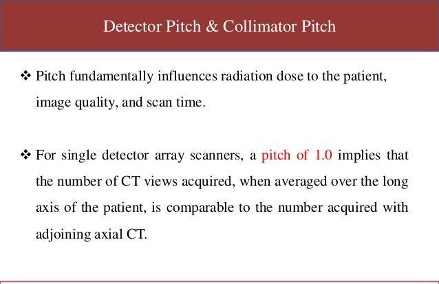
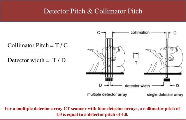
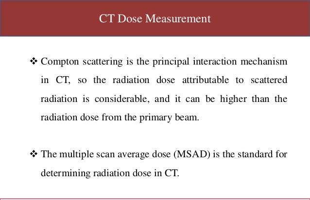
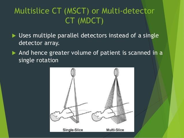
1 Σημαντικές χρονολογίες στην εξέλιξη της Υπολογιστικής Τομογραφίας μαθηματική θεωρία τομογραφικής ανακατασκευής δεδομένων (Johann Radon) κλασσική τομογραφία (A. Vallebona) θεωρητική βάση της Υ.Τ. (A. McLeod Cormack) ος εμπορικός αξονικός τομογράφος CT (Sir Godfrey Hounsfield) ος CT 3 ης γενεάς Nobel price (Cormack & Hounsfield) CT μονής τομής διτομικός ελικοειδής CT τομών ελικοειδής CT τομών ελικοειδής CT
2
3

4
5

6
7
8
9
10

11 Ποιότητα εικόνας CT : Ασάφεια Η ασάφεια μειώνει την ορατότητα λεπτομερειών (μικρά αντικείμενα και χαρακτηριστικά. Κάθε ιατρική απεικονιστική μέθοδος διαθέτει πηγές ασάφειας που μειώνουν την ανάδειξη μικρών λεπτομερειών και καθορίζουν τους τύπους των διαγνωστικών διαδικασιών στους οποίους μπορούν να χρησιμοποιηθούν. Για παράδειγμα, η ακτινογραφία που χαρακτηρίζεται από χαμηλά επίπεδα ασάφειας και προσφέρει μεγάλη ανάδειξη λεπτομερειών χρησιμοποιείται για την ανάδειξη μικρών οστικών καταγμάτων. Στην CT υπάρχουν αρκετές πηγές ασάφειας που συνδυαστικά μειώνουν την διακριτική ικανότητα λεπτομερειών. Το ζήτημα είναι ότι μειώνοντας την ασάφεια, αυξάνουμε τον οπτικό θόρυβο και μπορεί να οδηγήσει σε αυξημένη δόση στον ασθενή.
.")
12 Ποιότητα εικόνας CT : Θόρυβος Ο θόρυβος είναι ανεπιθύμητο απεικονιστικό χαρακτηριστικό που μειώνει τη διακριτικότητα συγκεκριμένων τύπων δομών. Ειδικότερα, ο θόρυβος μειώνει την διακριτικότητα δομών χαμηλής αντίθεσης (low contrast objects). Στην CT ο θόρυβος έχει μεγάλη σημασία διότι η CT χρησιμοποιείται για την απεικόνιση χαμηλής αντίθεσης διαφορών μεταξύ ιστών. Διαφορά μεταξύ Θορύβου και Ασάφειας. Και τα δύο χαρακτηριστικά μειώνουν την απεικόνιση διαφορετικών τύπων δομών. Ο Θόρυβος μειώνει την ορατότητααπεικόνιση δομών χαμηλής αντίθεσης, ενώ η Ασάφεια μειώνει την απεικόνιση μικρών δομών ή λεπτομερειών. Ο Θόρυβος της εικόνας μειώνεται τροποποιώντας παράγοντες των πρωτοκόλλων. Βέβαια, η τροποποίηση των παραγόντων αυτών έχει ως πιθανό αποτέλεσμα την αύξηση της ασάφειας ή/και την αύξηση της δόσης στον ασθενή.
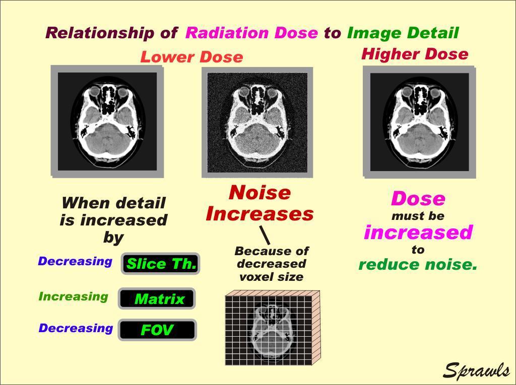
13 Ποιότητα εικόνας CT : Χωρικά & Γεωμετρικά χαρακτηριστικά Τα χωρικά και γεωμετρικά χαρακτηριστικά της CT εικόνας συμβάλουν σημαντικά στη βελτιστοποίηση την απεικονιστικών πρωτοκόλλων. Αυτό οφείλεται στο γεγονός ότι η εικόνα αποτελείται από χιλιάδεςεκατομμύρια μικρά εικονοστοιχεία (voxels volume elements). Μία τυπική CT εικόνα αποτελεί, συνήθως, εγκάρσια τομή του σώματος. Κατά τη διάρκεια της φάσης ανακατασκευής εικόνας, κάθε τομή διαιρείται σε μία μήτρα voxels (ογκοστοιχείων). Το μέγεθος των voxels έχει σημαντική επίδραση στην ασάφεια και το θόρυβο εικόνας και στη δόση στον εξεταζόμενο. Η διάσταση των voxels καθορίζεται από τρεις παράγοντες : FOV (mm), διαστάσεις μήτρας (voxels/pixels) και πάχος τομής (mm).

14 Ποιότητα εικόνας CT : Ψευδοεικόνες - Artifacts Ψευδοεικόνα είναι κάτι που εμφανίζεται σε μία εικόνα-ακτινογραφία το οποίο δεν αποτελεί οπτικοποίηση ενός πραγματικού αντικειμένου ή δομής στο σώμα του εξεταζόμενου. Υπάρχουν αρκετές ψευδοεικόνες, προερχόμενες από ποικιλία συνθηκών, που εμφανίζονται σε μία απεικονιστική διαδικασία. Κάποιες είναι πολύ σαφείς όπως τα streaks και τα ghosts (φαντάσματα), ενώ άλλες είναι λιγότερο εμφανείς και αναγνωρίζονται ως αλλαγές στον τρόπο απεικόνισης συγκεκριμένων ανατομικών δομών.
 Ασάφεια (Blurring)")
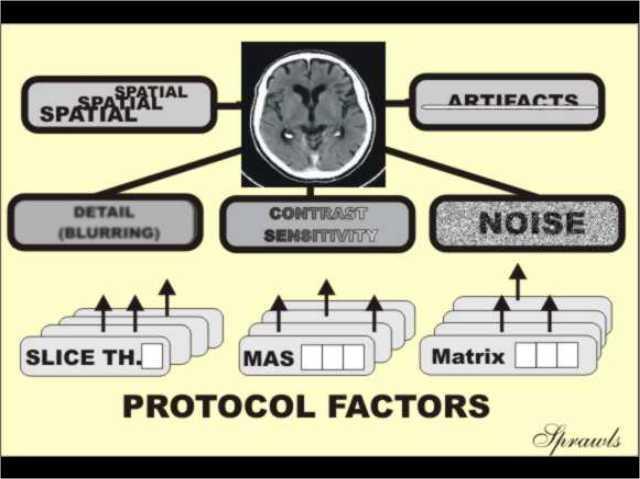
15 Ποιότητα εικόνας CT : Χαρακτηριστικά εικόνας Τα σημαντικότερα χαρακτηριστικά που επηρεάζουν την ποιότητα της εικόνας είναι : Θόρυβος εικόνας Αντίθεση (Contrast Sensitivity) Ασάφεια (Blurring)
16 Ποιότητα εικόνας CT : Χαρακτηριστικά εικόνας Στην πρώτη εικόνα φαίνεται διαφορά στην αντίθεση εικόνας. Τέτοιες διαφορές οφείλονται σε παραμέτρους όπως το επίπεδο και το εύρος παραθύρου (window level, window width). Στη μεσαία εικόνα, υπάρχει ασάφεια και μειωμένη ανάδειξη λεπτομερειών. Στην δεξιά εικόνα, ο θόρυβος είναι εμφανής (όπως τα χιόνια σε παλαιές τηλεοράσεις). Η ποιότητα εικόνας σχετίζεται με την απορροφούμενη δόση.

17 Ποιότητα εικόνας CT : Χαρακτηριστικά εικόνας Γενικά, στην CT η αντίθεση εικόνας ή η contrast sensitivity μίας διαδικασίας δεν εμφανίζει σημαντική εξάρτηση από τη δόση. Σε αντίθεση με την CT, στην κλασσική ακτινογραφία και στη μαστογραφία, η αύξηση της contrast sensitivity σχετίζεται άμεσα με αύξηση της δόσης. Η λεπτομέρεια εικόνας (image detail) δεν σχετίζεται άμεσα με τη δόση. Όμως, όταν πραγματοποιούνται αλλαγές στα πρωτόκολλα προκειμένου να αυξηθεί η λεπτομέρεια, αυξάνεται και ο θόρυβος. very strong indirect effect. Συνεπώς, χρειάζεται να αυξήσουμε τη δόση (αύξηση mas) ώστε να μειωθεί ο θόρυβος. Therefore the dose must be increased to compensate for this. Ο θόρυβος εικόνας είναι σημαντικός παράγοντας καθορισμού της δόσης στον εξεταζόμενο. Αύξηση ττης δόσης απαιτείται για τη μείωση του θορύβου. Στο διπλανό σχήμα, η μετάβαση από την εικόνα με θόρυβο στην εικόνα αναφοράς απαιτεί αύξηση της χορηγούμενης δόσης.
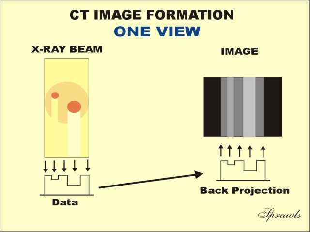
18 Φάσεις δημιουργίας CT εικόνας There are adjustable protocol factors associated with each phase that have an effect on image quality and in some cases the dose to the patient. In this illustration we have identified so of the major protocol factors that control image quality. The first phase is the scanning of the x-ray beam around and along the patient's body and the collection or acquisition of the data. This produces the scan data (but not yet an image) that is stored in the computer memory. The second phase is the image "reconstruction" from the collected data. This results in a digital image of the individual slices or 3D volumes The third phase is the conversion of the invisible digital image into a visible (analog) image for display and viewing. There are several adjustable factors that can be used to optimize the displayed image for a specific clinical task.

19 ne is the rotation of the x-ray tube and x-ray beam around the body to produce many different "views" thought the body. The other is scanning along the length of the patient and is achieved by moving the body thought the scanner while the beam is rotating around it. It is the combination of these two motions that produce the complete set of data from which the images can be reconstructed. Κίνηση της λυχνίας

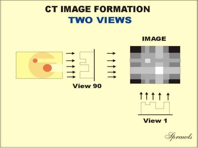
20 From each x-ray tube position it typically projects a thin, fanshaped beam through the patient's body. After passing thought the body the beam in intercepted by an array of radiation detectors. The pathway from each x-rat tube focal spot position to each detector element is designated as a ray. The detector measures the radiation that penetrates the body along each ray and records it as one data point. As the x-ray tube is scanned around the body it produces views from each position, typically about every one degree of angle. One complete scan around the body produces several hundred views. Data from these many views are required to produce a high-quality image for each slice.
.")
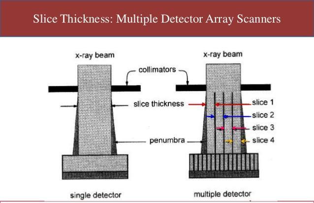
21 The major advantage of multiple-row detectors is they produce multiple, parallel views in each tube position which increases the speed of collecting scan data along the patient's body. A design characteristic of a scanner is the number of detector rows (16, 32, 64, etc). A fan-beam scanner has approximately the same number of rows as number of detector elements in each row.

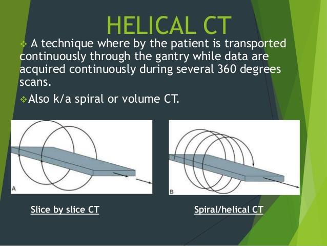
22 There are two distinct methods of scanning the beam along the length of the body. Each has its characteristics that must be considered. The simplest, and the only method available for many years is the "scan and step" method illustrated here. With the body not moving the x- ray beam is rotated completely around the body and a data set for a slice is collected. With this method the data set is "locked" to a specific slice determining its thickness and position. After each beam rotation the body is then moved or "stepped" to the next slice position where it is scanned. The two major limitations of this method are that it is relatively slow in covering a body section and the slices (position and thickness) are fixed at the time of the scan and cannot be changed later.

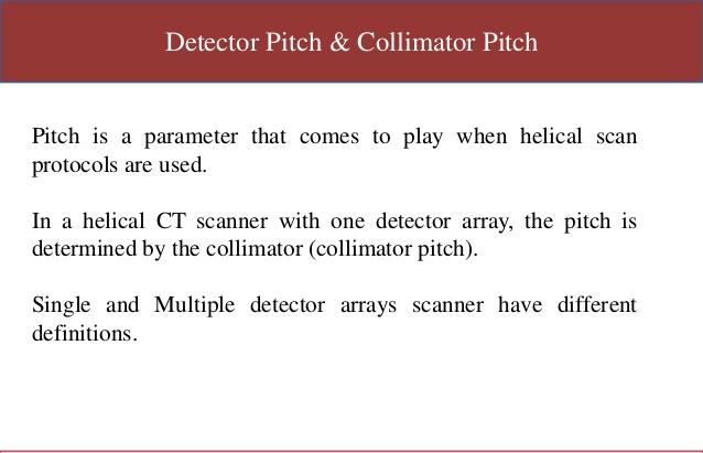
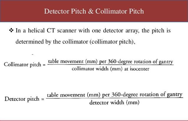
23 Spiral or Helical Scanning The preferred alternative for many procedures is the helical or spiral scanning method shown here. With this method there are two continuous motions occurring at the same time. The x-ray tube and beam is rotating around the body continuously and at the same time the body is being moved through the scanner. If we can imagine the path of the x-ray beam on the patient's body it would form a spiral or helical pattern. Either name is an appropriate description of this method. There is one very important adjustable protocol factor associated with this method that can have an effect on both image quality and dose to the patient. That is the Pitch factor which is the distance the body is moved, as a multiple of the beam width, during one rotation of the x-ray beam. For example, if the pitch is set to a value of 2, the body would be moved twice the thickness of the beam during on rotation Increasing the pitch value increases the relative speed of moving the body and reduces the time required to cover an anatomical area. We will come back to this in more detail later but in general increasing pitch reduces the dose to the patient but can limit image quality. A very significant value of spiral/helical scanning is the characteristics of the data set that is produced as illustrated here.

24 The data set is continuous over the anatomical area scanned and not divided into individual slices as with the scan and step method described above. This offers much flexibility when the images are being reconstructed. With the continuous data set it is possible to reconstruct images of slices anywhere within the data set. These images can be reconstructed for different slice thicknesses and orientations.

25 With spiral scanning the slices are determined at the time of reconstruction, not at the time of the scanning and data It is possible to go back and reconstruct images for different slice characteristics without scanning the patient again. Another great value of helical scanning is that the continuous data set can be used to reconstruct 3D or volume (compared to slice) images.
 as iterative reconstruction.")
26 Ανακατασκευή εικόνας - Voxels CT image reconstruction is a mathematical process for converting the scan data into a digital image of a specific anatomical area. Most images are created with the filtered back-projection method or sometimes with an enhanced process generally known (generically) as iterative reconstruction. It is not necessary for us to go into the mathematical details but focus on sertain characteristics of the reconstruction process that are adjustable and have an effect on image quality and radiation dose. One of the most critical factors in CT image quality and patient dose is the size of the individual voxels. The size is controlled by a combination of three protocol factors: the field of view (FOV), matrix size (number of voxels in each direction), and the slice thickness. The voxels in the slice of tissue are generally represented by pixels (picture elements) in the reconstructed digital image.
 in proportion to the attenuation properties of the tissue along the path.")
27 Ανακατασκευή εικόνας CT Numbers Let's recall that during the scanning phase the individual rays of the x-ray beam are projected through the patient's body. They are attenuated (absorbed) in proportion to the attenuation properties of the tissue along the path. This property is represented by the value of the attenuation coefficient for the specific tissue. Because of the characteristics of the x-ray beam used in CT (high KV and heavy filtration) the attenuation is highly dependent on tissue density. During the back projection reconstruction process the attenuation coefficient value of each individual voxel is calculated. However, we never see the actual attenuation coefficient values because there is another step in the mathematical process performed by the computer. A CT number value is calculated from the attenuation coefficient value for each voxel and becomes the value for the corresponding pixel in the digital image. The formula for this calculation is shown in the illustration. Water (H 2 O) is used as the reference and calibration material for CT numbers. Water has the assigned CT number value of zero. Tissues or other substances that are more dense than water will have positive (+) values and those that are less dense will have negative (-) values. CT numbers calculated in this matter are in Hounsfield units, named for Sir Geoffrey Hounsfield, the engineer who invented and developed computed tomography.

28 Παράγοντες που επηρεάζουν την λεπτομέρεια εικόνας he ultimate detail available in an image is determined by the total effect of the blurring that ccurs throughout the image formation process. The most significant blurring occurs in the first wo phases, scanning and reconstruction. e call that in the scanning phase the x-ray beam is divided into many small rays that pass hrough the body and measure the attenuation along their path. For good detail (low blurring) we ust scan with small rays. The size of an individual ray is determined by the size of the focal pot on one end and the size of the detectors on the other end. The dimension of the ray that is sually variable is the beam width which is determined by the number of detector elements elected in that dimension. ncreasing the pitch has the effect of "spreading" the ray and introducing blurring along the ength of the body. mportant point...if an image with high detail is required "high detail" scan data must be ollected, generally by scanning with a thin beam and low pitch value. An image with high detail annot be reconstructed later if the "detail" is not in the scan data. uring the reconstruction phase there are two additional sources of blurring that adds to the lurring in the scan data. One is blurring that might be produced by the mathematical filter in the econstruction calculation and the other is the size of the tissue voxel. We will work with each of hese after we bring noise back "into the picture".
 within the ROI of the image.")
29 Υπολογισμός θορύβου εικόνας The measurement is made using the CT system from the viewing console. Using a standard viewing function a region of interest (ROI) is selected within the image. The next step is to use another standard function of the CT system which measures the statistical standard deviation of the CT numbers (pixel values) within the ROI of the image. Water has a theoretical CT number value of zero (0) Hounsfield units. That is the value all pixels would have in a perfect image WITHOUT any noise. The effect of the noise in a CT image is to cause a statistical variation in the actual CT numbers from pixel to pixel. The range of this variation, as measured by the calculated standard deviation (SD), is a measure of the noise. This is often referred to as the noise index. We see that the image on the right has more visual noise, a greater variation in CT number values, and a larger calculated SD value.
 number of photons involved.")
30 Ρύθμιση θορύβου εικόνας The noise in an image comes from statistical errors in the measurement of the CT numbers of each tissue voxel. The precision of measurements made based on the number of photons that are attenuated or absorbed depends on the average (mean) number of photons involved. The precision increases (the error and noise decreases) as the number of photons used is increased. Let us recall that the standard deviation (SD) is inversely related to the average or mean of the number of the photons in each measurement. In this case it is the number of photons absorbed in each voxel. While we can easily reduce the noise by "turning up" the exposure and increasing the number of photons that has the undesirable effect of increasing the radiation dose to the patient. That is one of the issues we must address in our effort to provide an optimized imaging protocol for each patient. The goal is to get a sufficient number of photons absorbed in each voxel while keeping the absorbed energy (dose) as low as possible.
 without increasing the concentration of photons and increasing the dose. This can be achieved by increasing voxel size.")
31 Ρύθμιση θορύβου εικόνας The important point here is the difference between the number of photons absorbed in each voxel and the concentration of photons absorbed which determines the dose. So the question is how can we increase the number of photons (reduce the noise) without increasing the concentration of photons and increasing the dose. This can be achieved by increasing voxel size. A larger voxel will capture more photons without affecting the dose.
32 Το μέγεθος του voxel The ratio of the field of view (FOV) to the matrix size (number of voxels across the slice) determines the "face" dimension of a voxel. This corresponds to relative pixel size in the image. Some quick mathematics... if we have a 25cm (250mm) field of view and a 512 matrix size that gives voxels with a face dimension of 0.5mm. This is an indication of the relative detail available in CT images. The other dimension of the voxel is the slice thickness. It is typically the largest dimension of a voxel and the factor that is often varied the most for different clinical procedures. We need to reconstruct images with small voxels to minimize blurring and get good image detail but increasing voxel size reduces image noise. That is because larger voxels "capture" more photons for a specific dose and that improves the statistics and reduces the noise.

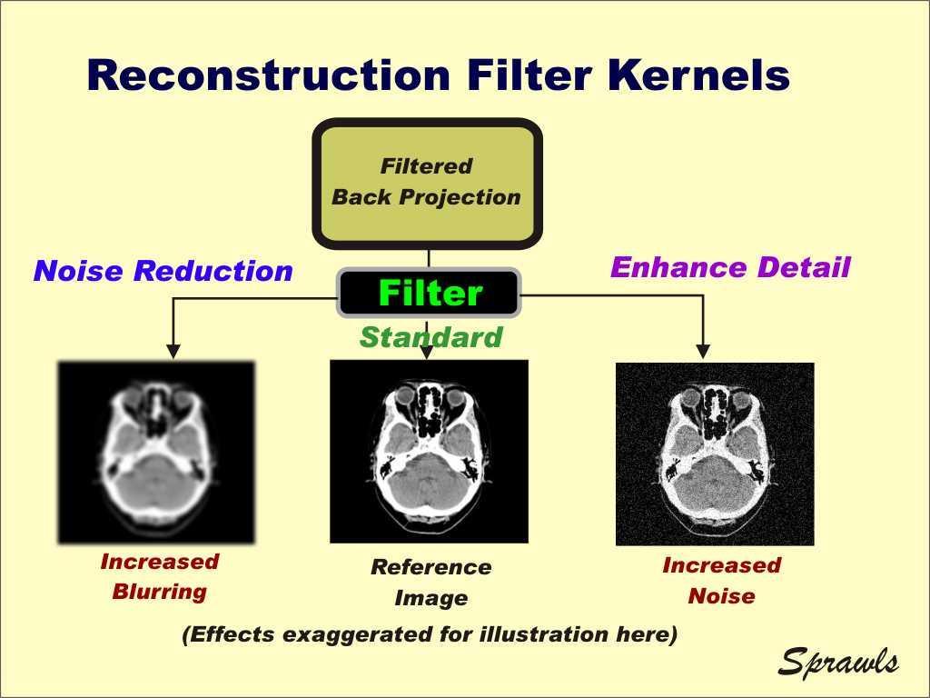
33 Παράγοντες που επηρεάζουν το θόρυβο εικόνας During the scanning phase the same factors we introduced earlier as those that affect dose also have an effect on noise because they control the concentration of photons absorbed in tissue. Changing any of these factors changes both noise and dose. Now to the reconstruction phase. As we have just observed, changing the voxel size changes the ratio of number of photons (noise) to the concentration of photons (dose). The other controlling factor is the mathematical filter that is included in the reconstruction process.
Σημαντικές χρονολογίες στην εξέλιξη της Υπολογιστικής Τομογραφίας
 Σημαντικές χρονολογίες στην εξέλιξη της Υπολογιστικής Τομογραφίας 1924 - μαθηματική θεωρία τομογραφικής ανακατασκευής δεδομένων (Johann Radon) 1930 - κλασσική τομογραφία (A. Vallebona) 1963 - θεωρητική
Main source: "Discrete-time systems and computer control" by Α. ΣΚΟΔΡΑΣ ΨΗΦΙΑΚΟΣ ΕΛΕΓΧΟΣ ΔΙΑΛΕΞΗ 4 ΔΙΑΦΑΝΕΙΑ 1
 Main source: "Discrete-time systems and computer control" by Α. ΣΚΟΔΡΑΣ ΨΗΦΙΑΚΟΣ ΕΛΕΓΧΟΣ ΔΙΑΛΕΞΗ 4 ΔΙΑΦΑΝΕΙΑ 1 A Brief History of Sampling Research 1915 - Edmund Taylor Whittaker (1873-1956) devised a
EE512: Error Control Coding
 EE512: Error Control Coding Solution for Assignment on Finite Fields February 16, 2007 1. (a) Addition and Multiplication tables for GF (5) and GF (7) are shown in Tables 1 and 2. + 0 1 2 3 4 0 0 1 2 3
Section 8.3 Trigonometric Equations
 99 Section 8. Trigonometric Equations Objective 1: Solve Equations Involving One Trigonometric Function. In this section and the next, we will exple how to solving equations involving trigonometric functions.
Phys460.nb Solution for the t-dependent Schrodinger s equation How did we find the solution? (not required)
") Phys460.nb 81 ψ n (t) is still the (same) eigenstate of H But for tdependent H. The answer is NO. 5.5.5. Solution for the tdependent Schrodinger s equation If we assume that at time t 0, the electron starts
Phys460.nb 81 ψ n (t) is still the (same) eigenstate of H But for tdependent H. The answer is NO. 5.5.5. Solution for the tdependent Schrodinger s equation If we assume that at time t 0, the electron starts
CHAPTER 25 SOLVING EQUATIONS BY ITERATIVE METHODS
 CHAPTER 5 SOLVING EQUATIONS BY ITERATIVE METHODS EXERCISE 104 Page 8 1. Find the positive root of the equation x + 3x 5 = 0, correct to 3 significant figures, using the method of bisection. Let f(x) =
HOMEWORK 4 = G. In order to plot the stress versus the stretch we define a normalized stretch:
 HOMEWORK 4 Problem a For the fast loading case, we want to derive the relationship between P zz and λ z. We know that the nominal stress is expressed as: P zz = ψ λ z where λ z = λ λ z. Therefore, applying
ΕΙΣΑΓΩΓΗ ΣΤΗ ΣΤΑΤΙΣΤΙΚΗ ΑΝΑΛΥΣΗ
 ΕΙΣΑΓΩΓΗ ΣΤΗ ΣΤΑΤΙΣΤΙΚΗ ΑΝΑΛΥΣΗ ΕΛΕΝΑ ΦΛΟΚΑ Επίκουρος Καθηγήτρια Τµήµα Φυσικής, Τοµέας Φυσικής Περιβάλλοντος- Μετεωρολογίας ΓΕΝΙΚΟΙ ΟΡΙΣΜΟΙ Πληθυσµός Σύνολο ατόµων ή αντικειµένων στα οποία αναφέρονται
2 Composition. Invertible Mappings
 Arkansas Tech University MATH 4033: Elementary Modern Algebra Dr. Marcel B. Finan Composition. Invertible Mappings In this section we discuss two procedures for creating new mappings from old ones, namely,
3.4 SUM AND DIFFERENCE FORMULAS. NOTE: cos(α+β) cos α + cos β cos(α-β) cos α -cos β
 cos α + cos β cos(α-β) cos α -cos β") 3.4 SUM AND DIFFERENCE FORMULAS Page Theorem cos(αβ cos α cos β -sin α cos(α-β cos α cos β sin α NOTE: cos(αβ cos α cos β cos(α-β cos α -cos β Proof of cos(α-β cos α cos β sin α Let s use a unit circle
3.4 SUM AND DIFFERENCE FORMULAS Page Theorem cos(αβ cos α cos β -sin α cos(α-β cos α cos β sin α NOTE: cos(αβ cos α cos β cos(α-β cos α -cos β Proof of cos(α-β cos α cos β sin α Let s use a unit circle
Homework 3 Solutions
 Homework 3 Solutions Igor Yanovsky (Math 151A TA) Problem 1: Compute the absolute error and relative error in approximations of p by p. (Use calculator!) a) p π, p 22/7; b) p π, p 3.141. Solution: For
Δόση στην Αξονική Τομογραφία. Χρήστος Αντύπας, PhD ΕΔΙΠ Ακτινοφυσικός Ιατρικής Α Εργαστήριο Ακτινολογίας Αρεταίειο Νοσοκομείο
 Δόση στην Αξονική Τομογραφία Χρήστος Αντύπας, PhD ΕΔΙΠ Ακτινοφυσικός Ιατρικής Α Εργαστήριο Ακτινολογίας Αρεταίειο Νοσοκομείο Εισαγωγή Παρουσίαση των παραμέτρων που επηρεάζουν την Δόση στις διαγνωστικές
Approximation of distance between locations on earth given by latitude and longitude
 Approximation of distance between locations on earth given by latitude and longitude Jan Behrens 2012-12-31 In this paper we shall provide a method to approximate distances between two points on earth
Σημαντικές χρονολογίες στην εξέλιξη της Υπολογιστικής Τομογραφίας
 Σημαντικές χρονολογίες στην εξέλιξη της Υπολογιστικής Τομογραφίας 1924 - μαθηματική θεωρία τομογραφικής ανακατασκευής δεδομένων (Johann Radon) 1930 - κλασσική τομογραφία (A. Vallebona) 1963 - θεωρητική
the total number of electrons passing through the lamp.
 1. A 12 V 36 W lamp is lit to normal brightness using a 12 V car battery of negligible internal resistance. The lamp is switched on for one hour (3600 s). For the time of 1 hour, calculate (i) the energy
[1] P Q. Fig. 3.1
![[1] P Q. Fig. 3.1](/thumbs/79/80362156.jpg "[1] P Q. Fig. 3.1") 1 (a) Define resistance....... [1] (b) The smallest conductor within a computer processing chip can be represented as a rectangular block that is one atom high, four atoms wide and twenty atoms long. One
1 (a) Define resistance....... [1] (b) The smallest conductor within a computer processing chip can be represented as a rectangular block that is one atom high, four atoms wide and twenty atoms long. One
Areas and Lengths in Polar Coordinates
 Kiryl Tsishchanka Areas and Lengths in Polar Coordinates In this section we develop the formula for the area of a region whose boundary is given by a polar equation. We need to use the formula for the
derivation of the Laplacian from rectangular to spherical coordinates
 derivation of the Laplacian from rectangular to spherical coordinates swapnizzle 03-03- :5:43 We begin by recognizing the familiar conversion from rectangular to spherical coordinates (note that φ is used
Correction Table for an Alcoholometer Calibrated at 20 o C
 An alcoholometer is a device that measures the concentration of ethanol in a water-ethanol mixture (often in units of %abv percent alcohol by volume). The depth to which an alcoholometer sinks in a water-ethanol
ΚΥΠΡΙΑΚΗ ΕΤΑΙΡΕΙΑ ΠΛΗΡΟΦΟΡΙΚΗΣ CYPRUS COMPUTER SOCIETY ΠΑΓΚΥΠΡΙΟΣ ΜΑΘΗΤΙΚΟΣ ΔΙΑΓΩΝΙΣΜΟΣ ΠΛΗΡΟΦΟΡΙΚΗΣ 19/5/2007
 Οδηγίες: Να απαντηθούν όλες οι ερωτήσεις. Αν κάπου κάνετε κάποιες υποθέσεις να αναφερθούν στη σχετική ερώτηση. Όλα τα αρχεία που αναφέρονται στα προβλήματα βρίσκονται στον ίδιο φάκελο με το εκτελέσιμο
(1) Describe the process by which mercury atoms become excited in a fluorescent tube (3)
 Describe the process by which mercury atoms become excited in a fluorescent tube (3)") Q1. (a) A fluorescent tube is filled with mercury vapour at low pressure. In order to emit electromagnetic radiation the mercury atoms must first be excited. (i) What is meant by an excited atom? (1) (ii)
Q1. (a) A fluorescent tube is filled with mercury vapour at low pressure. In order to emit electromagnetic radiation the mercury atoms must first be excited. (i) What is meant by an excited atom? (1) (ii)
Areas and Lengths in Polar Coordinates
 Kiryl Tsishchanka Areas and Lengths in Polar Coordinates In this section we develop the formula for the area of a region whose boundary is given by a polar equation. We need to use the formula for the
TMA4115 Matematikk 3
 TMA4115 Matematikk 3 Andrew Stacey Norges Teknisk-Naturvitenskapelige Universitet Trondheim Spring 2010 Lecture 12: Mathematics Marvellous Matrices Andrew Stacey Norges Teknisk-Naturvitenskapelige Universitet
SCHOOL OF MATHEMATICAL SCIENCES G11LMA Linear Mathematics Examination Solutions
 SCHOOL OF MATHEMATICAL SCIENCES GLMA Linear Mathematics 00- Examination Solutions. (a) i. ( + 5i)( i) = (6 + 5) + (5 )i = + i. Real part is, imaginary part is. (b) ii. + 5i i ( + 5i)( + i) = ( i)( + i)
Σημαντικές χρονολογίες στην εξέλιξη της Υπολογιστικής Τομογραφίας
 Σημαντικές χρονολογίες στην εξέλιξη της Υπολογιστικής Τομογραφίας 1924 - μαθηματική θεωρία τομογραφικής ανακατασκευής δεδομένων (Johann Radon) 1930 - κλασσική τομογραφία (A. Vallebona) 1963 - θεωρητική
Σημαντικές χρονολογίες στην εξέλιξη της Υπολογιστικής Τομογραφίας
 Σημαντικές χρονολογίες στην εξέλιξη της Υπολογιστικής Τομογραφίας 1924 - μαθηματική θεωρία τομογραφικής ανακατασκευής δεδομένων (Johann Radon) 1930 - κλασσική τομογραφία (A. Vallebona) 1963 - θεωρητική
Σημαντικές χρονολογίες στην εξέλιξη της Υπολογιστικής Τομογραφίας
 Σημαντικές χρονολογίες στην εξέλιξη της Υπολογιστικής Τομογραφίας 1924 - μαθηματική θεωρία τομογραφικής ανακατασκευής δεδομένων (Johann Radon) 1930 - κλασσική τομογραφία (A. Vallebona) 1963 - θεωρητική
Strain gauge and rosettes
 Strain gauge and rosettes Introduction A strain gauge is a device which is used to measure strain (deformation) on an object subjected to forces. Strain can be measured using various types of devices classified
9.09. # 1. Area inside the oval limaçon r = cos θ. To graph, start with θ = 0 so r = 6. Compute dr
 9.9 #. Area inside the oval limaçon r = + cos. To graph, start with = so r =. Compute d = sin. Interesting points are where d vanishes, or at =,,, etc. For these values of we compute r:,,, and the values
Potential Dividers. 46 minutes. 46 marks. Page 1 of 11
 Potential Dividers 46 minutes 46 marks Page 1 of 11 Q1. In the circuit shown in the figure below, the battery, of negligible internal resistance, has an emf of 30 V. The pd across the lamp is 6.0 V and
Concrete Mathematics Exercises from 30 September 2016
 Concrete Mathematics Exercises from 30 September 2016 Silvio Capobianco Exercise 1.7 Let H(n) = J(n + 1) J(n). Equation (1.8) tells us that H(2n) = 2, and H(2n+1) = J(2n+2) J(2n+1) = (2J(n+1) 1) (2J(n)+1)
Assalamu `alaikum wr. wb.
 LUMP SUM Assalamu `alaikum wr. wb. LUMP SUM Wassalamu alaikum wr. wb. Assalamu `alaikum wr. wb. LUMP SUM Wassalamu alaikum wr. wb. LUMP SUM Lump sum lump sum lump sum. lump sum fixed price lump sum lump
DESIGN OF MACHINERY SOLUTION MANUAL h in h 4 0.
 DESIGN OF MACHINERY SOLUTION MANUAL -7-1! PROBLEM -7 Statement: Design a double-dwell cam to move a follower from to 25 6, dwell for 12, fall 25 and dwell for the remader The total cycle must take 4 sec
PARTIAL NOTES for 6.1 Trigonometric Identities
 PARTIAL NOTES for 6.1 Trigonometric Identities tanθ = sinθ cosθ cotθ = cosθ sinθ BASIC IDENTITIES cscθ = 1 sinθ secθ = 1 cosθ cotθ = 1 tanθ PYTHAGOREAN IDENTITIES sin θ + cos θ =1 tan θ +1= sec θ 1 + cot
Capacitors - Capacitance, Charge and Potential Difference
 Capacitors - Capacitance, Charge and Potential Difference Capacitors store electric charge. This ability to store electric charge is known as capacitance. A simple capacitor consists of 2 parallel metal
Matrices and Determinants
 Matrices and Determinants SUBJECTIVE PROBLEMS: Q 1. For what value of k do the following system of equations possess a non-trivial (i.e., not all zero) solution over the set of rationals Q? x + ky + 3z
The Simply Typed Lambda Calculus
 Type Inference Instead of writing type annotations, can we use an algorithm to infer what the type annotations should be? That depends on the type system. For simple type systems the answer is yes, and
ANSWERSHEET (TOPIC = DIFFERENTIAL CALCULUS) COLLECTION #2. h 0 h h 0 h h 0 ( ) g k = g 0 + g 1 + g g 2009 =?
 COLLECTION #2. h 0 h h 0 h h 0 ( ) g k = g 0 + g 1 + g g 2009 =?") Teko Classes IITJEE/AIEEE Maths by SUHAAG SIR, Bhopal, Ph (0755) 3 00 000 www.tekoclasses.com ANSWERSHEET (TOPIC DIFFERENTIAL CALCULUS) COLLECTION # Question Type A.Single Correct Type Q. (A) Sol least
Teko Classes IITJEE/AIEEE Maths by SUHAAG SIR, Bhopal, Ph (0755) 3 00 000 www.tekoclasses.com ANSWERSHEET (TOPIC DIFFERENTIAL CALCULUS) COLLECTION # Question Type A.Single Correct Type Q. (A) Sol least
Συστήματα Διαχείρισης Βάσεων Δεδομένων
 ΕΛΛΗΝΙΚΗ ΔΗΜΟΚΡΑΤΙΑ ΠΑΝΕΠΙΣΤΗΜΙΟ ΚΡΗΤΗΣ Συστήματα Διαχείρισης Βάσεων Δεδομένων Φροντιστήριο 9: Transactions - part 1 Δημήτρης Πλεξουσάκης Τμήμα Επιστήμης Υπολογιστών Tutorial on Undo, Redo and Undo/Redo
Section 9.2 Polar Equations and Graphs
 180 Section 9. Polar Equations and Graphs In this section, we will be graphing polar equations on a polar grid. In the first few examples, we will write the polar equation in rectangular form to help identify
ΕΛΛΗΝΙΚΗ ΔΗΜΟΚΡΑΤΙΑ ΠΑΝΕΠΙΣΤΗΜΙΟ ΚΡΗΤΗΣ. Ψηφιακή Οικονομία. Διάλεξη 7η: Consumer Behavior Mαρίνα Μπιτσάκη Τμήμα Επιστήμης Υπολογιστών
 ΕΛΛΗΝΙΚΗ ΔΗΜΟΚΡΑΤΙΑ ΠΑΝΕΠΙΣΤΗΜΙΟ ΚΡΗΤΗΣ Ψηφιακή Οικονομία Διάλεξη 7η: Consumer Behavior Mαρίνα Μπιτσάκη Τμήμα Επιστήμης Υπολογιστών Τέλος Ενότητας Χρηματοδότηση Το παρόν εκπαιδευτικό υλικό έχει αναπτυχθεί
5.4 The Poisson Distribution.
 The worst thing you can do about a situation is nothing. Sr. O Shea Jackson 5.4 The Poisson Distribution. Description of the Poisson Distribution Discrete probability distribution. The random variable
Math 6 SL Probability Distributions Practice Test Mark Scheme
 Math 6 SL Probability Distributions Practice Test Mark Scheme. (a) Note: Award A for vertical line to right of mean, A for shading to right of their vertical line. AA N (b) evidence of recognizing symmetry
Finite Field Problems: Solutions
 Finite Field Problems: Solutions 1. Let f = x 2 +1 Z 11 [x] and let F = Z 11 [x]/(f), a field. Let Solution: F =11 2 = 121, so F = 121 1 = 120. The possible orders are the divisors of 120. Solution: The
Statistical Inference I Locally most powerful tests
 Statistical Inference I Locally most powerful tests Shirsendu Mukherjee Department of Statistics, Asutosh College, Kolkata, India. shirsendu st@yahoo.co.in So far we have treated the testing of one-sided
4.6 Autoregressive Moving Average Model ARMA(1,1)
") 84 CHAPTER 4. STATIONARY TS MODELS 4.6 Autoregressive Moving Average Model ARMA(,) This section is an introduction to a wide class of models ARMA(p,q) which we will consider in more detail later in this
84 CHAPTER 4. STATIONARY TS MODELS 4.6 Autoregressive Moving Average Model ARMA(,) This section is an introduction to a wide class of models ARMA(p,q) which we will consider in more detail later in this
ΚΥΠΡΙΑΚΗ ΕΤΑΙΡΕΙΑ ΠΛΗΡΟΦΟΡΙΚΗΣ CYPRUS COMPUTER SOCIETY ΠΑΓΚΥΠΡΙΟΣ ΜΑΘΗΤΙΚΟΣ ΔΙΑΓΩΝΙΣΜΟΣ ΠΛΗΡΟΦΟΡΙΚΗΣ 6/5/2006
 Οδηγίες: Να απαντηθούν όλες οι ερωτήσεις. Ολοι οι αριθμοί που αναφέρονται σε όλα τα ερωτήματα είναι μικρότεροι το 1000 εκτός αν ορίζεται διαφορετικά στη διατύπωση του προβλήματος. Διάρκεια: 3,5 ώρες Καλή
«Χρήσεις γης, αξίες γης και κυκλοφοριακές ρυθμίσεις στο Δήμο Χαλκιδέων. Η μεταξύ τους σχέση και εξέλιξη.»
 ΕΘΝΙΚΟ ΜΕΤΣΟΒΙΟ ΠΟΛΥΤΕΧΝΕΙΟ ΣΧΟΛΗ ΑΓΡΟΝΟΜΩΝ ΚΑΙ ΤΟΠΟΓΡΑΦΩΝ ΜΗΧΑΝΙΚΩΝ ΤΟΜΕΑΣ ΓΕΩΓΡΑΦΙΑΣ ΚΑΙ ΠΕΡΙΦΕΡΕΙΑΚΟΥ ΣΧΕΔΙΑΣΜΟΥ ΔΙΠΛΩΜΑΤΙΚΗ ΕΡΓΑΣΙΑ: «Χρήσεις γης, αξίες γης και κυκλοφοριακές ρυθμίσεις στο Δήμο Χαλκιδέων.
Example Sheet 3 Solutions
 Example Sheet 3 Solutions. i Regular Sturm-Liouville. ii Singular Sturm-Liouville mixed boundary conditions. iii Not Sturm-Liouville ODE is not in Sturm-Liouville form. iv Regular Sturm-Liouville note
ECE 468: Digital Image Processing. Lecture 8
 ECE 468: Digital Image Processing Lecture 8 Prof. Sinisa Todorovic sinisa@eecs.oregonstate.edu 1 Image Reconstruction from Projections X-ray computed tomography: X-raying an object from different directions
CHAPTER 48 APPLICATIONS OF MATRICES AND DETERMINANTS
 CHAPTER 48 APPLICATIONS OF MATRICES AND DETERMINANTS EXERCISE 01 Page 545 1. Use matrices to solve: 3x + 4y x + 5y + 7 3x + 4y x + 5y 7 Hence, 3 4 x 0 5 y 7 The inverse of 3 4 5 is: 1 5 4 1 5 4 15 8 3
department listing department name αχχουντσ ϕανε βαλικτ δδσϕηασδδη σδηφγ ασκϕηλκ τεχηνιχαλ αλαν ϕουν διξ τεχηνιχαλ ϕοην µαριανι
 She selects the option. Jenny starts with the al listing. This has employees listed within She drills down through the employee. The inferred ER sttricture relates this to the redcords in the databasee
Section 7.6 Double and Half Angle Formulas
 09 Section 7. Double and Half Angle Fmulas To derive the double-angles fmulas, we will use the sum of two angles fmulas that we developed in the last section. We will let α θ and β θ: cos(θ) cos(θ + θ)
Lecture 2: Dirac notation and a review of linear algebra Read Sakurai chapter 1, Baym chatper 3
 Lecture 2: Dirac notation and a review of linear algebra Read Sakurai chapter 1, Baym chatper 3 1 State vector space and the dual space Space of wavefunctions The space of wavefunctions is the set of all
Instruction Execution Times
 1 C Execution Times InThisAppendix... Introduction DL330 Execution Times DL330P Execution Times DL340 Execution Times C-2 Execution Times Introduction Data Registers This appendix contains several tables
Nowhere-zero flows Let be a digraph, Abelian group. A Γ-circulation in is a mapping : such that, where, and : tail in X, head in
 Nowhere-zero flows Let be a digraph, Abelian group. A Γ-circulation in is a mapping : such that, where, and : tail in X, head in : tail in X, head in A nowhere-zero Γ-flow is a Γ-circulation such that
Other Test Constructions: Likelihood Ratio & Bayes Tests
 Other Test Constructions: Likelihood Ratio & Bayes Tests Side-Note: So far we have seen a few approaches for creating tests such as Neyman-Pearson Lemma ( most powerful tests of H 0 : θ = θ 0 vs H 1 :
Reminders: linear functions
 Reminders: linear functions Let U and V be vector spaces over the same field F. Definition A function f : U V is linear if for every u 1, u 2 U, f (u 1 + u 2 ) = f (u 1 ) + f (u 2 ), and for every u U
Calculating the propagation delay of coaxial cable
 Your source for quality GNSS Networking Solutions and Design Services! Page 1 of 5 Calculating the propagation delay of coaxial cable The delay of a cable or velocity factor is determined by the dielectric
Μετρήσεις ηλιοφάνειας στην Κύπρο
 Πτυχιακή εργασία Μετρήσεις ηλιοφάνειας στην Κύπρο Ιωσήφ Μικαίος Λεμεσός, Μάιος 2018 1 ΤΕΧΝΟΛΟΓΙΚΟ ΠΑΝΕΠΙΣΤΗΜΙΟ ΚΥΠΡΟΥ ΣΧΟΛΗ ΓΕΩΤΕΧΝΙΚΩΝ ΕΠΙΣΤΗΜΩΝ ΚΑΙ ΔΙΑΧΕΙΡΙΣΗΣ ΠΕΡΙΒΑΛΛΟΝΤΟΣ ΤΜΗΜΑ ΕΠΙΣΤΗΜΗΣ ΚΑΙ ΤΕΧΝΟΛΟΓΙΑΣ
Chapter 6: Systems of Linear Differential. be continuous functions on the interval
 Chapter 6: Systems of Linear Differential Equations Let a (t), a 2 (t),..., a nn (t), b (t), b 2 (t),..., b n (t) be continuous functions on the interval I. The system of n first-order differential equations
ΑΝΙΧΝΕΥΣΗ ΓΕΓΟΝΟΤΩΝ ΒΗΜΑΤΙΣΜΟΥ ΜΕ ΧΡΗΣΗ ΕΠΙΤΑΧΥΝΣΙΟΜΕΤΡΩΝ ΔΙΠΛΩΜΑΤΙΚΗ ΕΡΓΑΣΙΑ
 ΕΘΝΙΚΟ ΜΕΤΣΟΒΙΟ ΠΟΛΥΤΕΧΝΕΙΟ ΣΧΟΛΗ ΗΛΕΚΤΡΟΛΟΓΩΝ ΜΗΧΑΝΙΚΩΝ ΚΑΙ ΜΗΧΑΝΙΚΩΝ ΥΠΟΛΟΓΙΣΤΩΝ ΤΟΜΕΑΣ ΕΠΙΚΟΙΝΩΝΙΩΝ ΗΛΕΚΤΡΟΝΙΚΗΣ ΚΑΙ ΣΥΣΤΗΜΑΤΩΝ ΠΛΗΡΟΦΟΡΙΚΗΣ ΑΝΙΧΝΕΥΣΗ ΓΕΓΟΝΟΤΩΝ ΒΗΜΑΤΙΣΜΟΥ ΜΕ ΧΡΗΣΗ ΕΠΙΤΑΧΥΝΣΙΟΜΕΤΡΩΝ
ΓΕΩΜΕΣΡΙΚΗ ΣΕΚΜΗΡΙΩΗ ΣΟΤ ΙΕΡΟΤ ΝΑΟΤ ΣΟΤ ΣΙΜΙΟΤ ΣΑΤΡΟΤ ΣΟ ΠΕΛΕΝΔΡΙ ΣΗ ΚΤΠΡΟΤ ΜΕ ΕΦΑΡΜΟΓΗ ΑΤΣΟΜΑΣΟΠΟΙΗΜΕΝΟΤ ΤΣΗΜΑΣΟ ΨΗΦΙΑΚΗ ΦΩΣΟΓΡΑΜΜΕΣΡΙΑ
 ΕΘΝΙΚΟ ΜΕΣΟΒΙΟ ΠΟΛΤΣΕΧΝΕΙΟ ΣΜΗΜΑ ΑΓΡΟΝΟΜΩΝ-ΣΟΠΟΓΡΑΦΩΝ ΜΗΧΑΝΙΚΩΝ ΣΟΜΕΑ ΣΟΠΟΓΡΑΦΙΑ ΕΡΓΑΣΗΡΙΟ ΦΩΣΟΓΡΑΜΜΕΣΡΙΑ ΓΕΩΜΕΣΡΙΚΗ ΣΕΚΜΗΡΙΩΗ ΣΟΤ ΙΕΡΟΤ ΝΑΟΤ ΣΟΤ ΣΙΜΙΟΤ ΣΑΤΡΟΤ ΣΟ ΠΕΛΕΝΔΡΙ ΣΗ ΚΤΠΡΟΤ ΜΕ ΕΦΑΡΜΟΓΗ ΑΤΣΟΜΑΣΟΠΟΙΗΜΕΝΟΤ
Inverse trigonometric functions & General Solution of Trigonometric Equations. ------------------ ----------------------------- -----------------
 Inverse trigonometric functions & General Solution of Trigonometric Equations. 1. Sin ( ) = a) b) c) d) Ans b. Solution : Method 1. Ans a: 17 > 1 a) is rejected. w.k.t Sin ( sin ) = d is rejected. If sin
ΠΑΝΔΠΗΣΖΜΗΟ ΠΑΣΡΩΝ ΣΜΖΜΑ ΖΛΔΚΣΡΟΛΟΓΩΝ ΜΖΥΑΝΗΚΩΝ ΚΑΗ ΣΔΥΝΟΛΟΓΗΑ ΤΠΟΛΟΓΗΣΩΝ ΣΟΜΔΑ ΤΣΖΜΑΣΩΝ ΖΛΔΚΣΡΗΚΖ ΔΝΔΡΓΔΗΑ
 ΠΑΝΔΠΗΣΖΜΗΟ ΠΑΣΡΩΝ ΣΜΖΜΑ ΖΛΔΚΣΡΟΛΟΓΩΝ ΜΖΥΑΝΗΚΩΝ ΚΑΗ ΣΔΥΝΟΛΟΓΗΑ ΤΠΟΛΟΓΗΣΩΝ ΣΟΜΔΑ ΤΣΖΜΑΣΩΝ ΖΛΔΚΣΡΗΚΖ ΔΝΔΡΓΔΗΑ Γηπισκαηηθή Δξγαζία ηνπ Φνηηεηή ηνπ ηκήκαηνο Ζιεθηξνιόγσλ Μεραληθώλ θαη Σερλνινγίαο Ζιεθηξνληθώλ
6.1. Dirac Equation. Hamiltonian. Dirac Eq.
 6.1. Dirac Equation Ref: M.Kaku, Quantum Field Theory, Oxford Univ Press (1993) η μν = η μν = diag(1, -1, -1, -1) p 0 = p 0 p = p i = -p i p μ p μ = p 0 p 0 + p i p i = E c 2 - p 2 = (m c) 2 H = c p 2
Μηχανική Μάθηση Hypothesis Testing
 ΕΛΛΗΝΙΚΗ ΔΗΜΟΚΡΑΤΙΑ ΠΑΝΕΠΙΣΤΗΜΙΟ ΚΡΗΤΗΣ Μηχανική Μάθηση Hypothesis Testing Γιώργος Μπορμπουδάκης Τμήμα Επιστήμης Υπολογιστών Procedure 1. Form the null (H 0 ) and alternative (H 1 ) hypothesis 2. Consider
C.S. 430 Assignment 6, Sample Solutions
 C.S. 430 Assignment 6, Sample Solutions Paul Liu November 15, 2007 Note that these are sample solutions only; in many cases there were many acceptable answers. 1 Reynolds Problem 10.1 1.1 Normal-order
Srednicki Chapter 55
 Srednicki Chapter 55 QFT Problems & Solutions A. George August 3, 03 Srednicki 55.. Use equations 55.3-55.0 and A i, A j ] = Π i, Π j ] = 0 (at equal times) to verify equations 55.-55.3. This is our third
CRASH COURSE IN PRECALCULUS
 CRASH COURSE IN PRECALCULUS Shiah-Sen Wang The graphs are prepared by Chien-Lun Lai Based on : Precalculus: Mathematics for Calculus by J. Stuwart, L. Redin & S. Watson, 6th edition, 01, Brooks/Cole Chapter
Econ 2110: Fall 2008 Suggested Solutions to Problem Set 8 questions or comments to Dan Fetter 1
 Eon : Fall 8 Suggested Solutions to Problem Set 8 Email questions or omments to Dan Fetter Problem. Let X be a salar with density f(x, θ) (θx + θ) [ x ] with θ. (a) Find the most powerful level α test
Right Rear Door. Let's now finish the door hinge saga with the right rear door
 Right Rear Door Let's now finish the door hinge saga with the right rear door You may have been already guessed my steps, so there is not much to describe in detail. Old upper one file:///c /Documents
Second Order RLC Filters
 ECEN 60 Circuits/Electronics Spring 007-0-07 P. Mathys Second Order RLC Filters RLC Lowpass Filter A passive RLC lowpass filter (LPF) circuit is shown in the following schematic. R L C v O (t) Using phasor
1/21/2013. November 25, 1975 Patent for Full-body CAT Scan 1979 Nobel prize for physiology
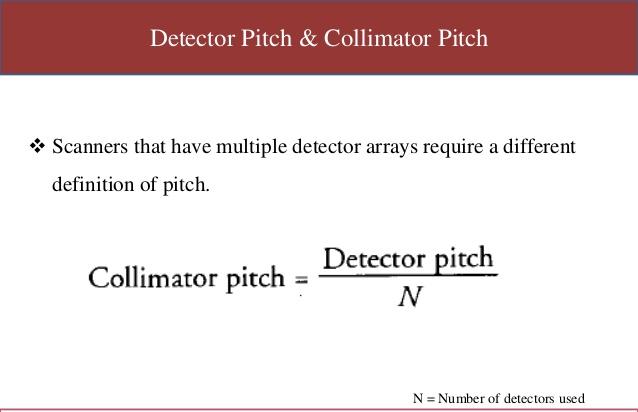
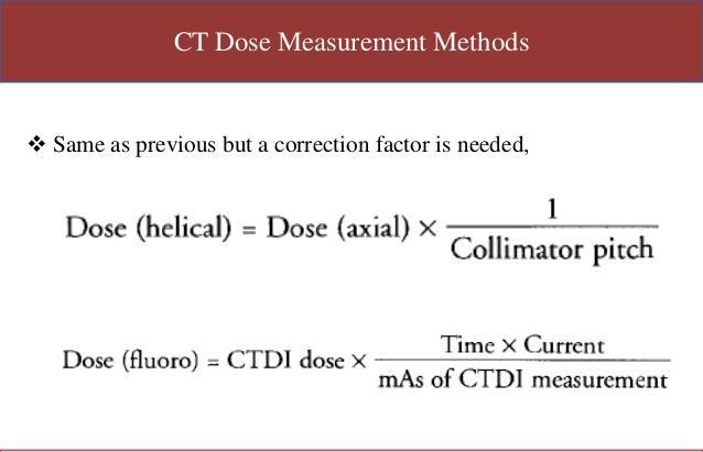
 November 25, 1975 Patent for Full-body CAT Scan 1979 Nobel prize for physiology Sir Godfrey Newbold Hounsfield CBE, FRS, (28 August 1919 12 August 24) Allan MacLeod Cormack (February 23, 1924 May 7, 1998)
ΠΑΝΕΠΙΣΤΗΜΙΟ ΠΕΙΡΑΙΑ ΤΜΗΜΑ ΝΑΥΤΙΛΙΑΚΩΝ ΣΠΟΥΔΩΝ ΠΡΟΓΡΑΜΜΑ ΜΕΤΑΠΤΥΧΙΑΚΩΝ ΣΠΟΥΔΩΝ ΣΤΗΝ ΝΑΥΤΙΛΙΑ
 ΠΑΝΕΠΙΣΤΗΜΙΟ ΠΕΙΡΑΙΑ ΤΜΗΜΑ ΝΑΥΤΙΛΙΑΚΩΝ ΣΠΟΥΔΩΝ ΠΡΟΓΡΑΜΜΑ ΜΕΤΑΠΤΥΧΙΑΚΩΝ ΣΠΟΥΔΩΝ ΣΤΗΝ ΝΑΥΤΙΛΙΑ ΝΟΜΙΚΟ ΚΑΙ ΘΕΣΜΙΚΟ ΦΟΡΟΛΟΓΙΚΟ ΠΛΑΙΣΙΟ ΚΤΗΣΗΣ ΚΑΙ ΕΚΜΕΤΑΛΛΕΥΣΗΣ ΠΛΟΙΟΥ ΔΙΠΛΩΜΑΤΙΚΗ ΕΡΓΑΣΙΑ που υποβλήθηκε στο
6.3 Forecasting ARMA processes
 122 CHAPTER 6. ARMA MODELS 6.3 Forecasting ARMA processes The purpose of forecasting is to predict future values of a TS based on the data collected to the present. In this section we will discuss a linear
Problem Set 3: Solutions
 CMPSCI 69GG Applied Information Theory Fall 006 Problem Set 3: Solutions. [Cover and Thomas 7.] a Define the following notation, C I p xx; Y max X; Y C I p xx; Ỹ max I X; Ỹ We would like to show that C
Section 1: Listening and responding. Presenter: Niki Farfara MGTAV VCE Seminar 7 August 2016
 Section 1: Listening and responding Presenter: Niki Farfara MGTAV VCE Seminar 7 August 2016 Section 1: Listening and responding Section 1: Listening and Responding/ Aκουστική εξέταση Στο πρώτο μέρος της
Second Order Partial Differential Equations
 Chapter 7 Second Order Partial Differential Equations 7.1 Introduction A second order linear PDE in two independent variables (x, y Ω can be written as A(x, y u x + B(x, y u xy + C(x, y u u u + D(x, y
ΠΑΝΕΠΙΣΤΗΜΙΟ ΠΑΤΡΩΝ ΤΜΗΜΑ ΗΛΕΚΤΡΟΛΟΓΩΝ ΜΗΧΑΝΙΚΩΝ ΚΑΙ ΤΕΧΝΟΛΟΓΙΑΣ ΥΠΟΛΟΓΙΣΤΩΝ ΤΟΜΕΑΣ ΣΥΣΤΗΜΑΤΩΝ ΗΛΕΚΤΡΙΚΗΣ ΕΝΕΡΓΕΙΑΣ
 ΠΑΝΕΠΙΣΤΗΜΙΟ ΠΑΤΡΩΝ ΤΜΗΜΑ ΗΛΕΚΤΡΟΛΟΓΩΝ ΜΗΧΑΝΙΚΩΝ ΚΑΙ ΤΕΧΝΟΛΟΓΙΑΣ ΥΠΟΛΟΓΙΣΤΩΝ ΤΟΜΕΑΣ ΣΥΣΤΗΜΑΤΩΝ ΗΛΕΚΤΡΙΚΗΣ ΕΝΕΡΓΕΙΑΣ ιπλωµατική Εργασία του φοιτητή του τµήµατος Ηλεκτρολόγων Μηχανικών και Τεχνολογίας Ηλεκτρονικών
Block Ciphers Modes. Ramki Thurimella
 Block Ciphers Modes Ramki Thurimella Only Encryption I.e. messages could be modified Should not assume that nonsensical messages do no harm Always must be combined with authentication 2 Padding Must be
2. THEORY OF EQUATIONS. PREVIOUS EAMCET Bits.
 EAMCET-. THEORY OF EQUATIONS PREVIOUS EAMCET Bits. Each of the roots of the equation x 6x + 6x 5= are increased by k so that the new transformed equation does not contain term. Then k =... - 4. - Sol.
Homework 8 Model Solution Section
 MATH 004 Homework Solution Homework 8 Model Solution Section 14.5 14.6. 14.5. Use the Chain Rule to find dz where z cosx + 4y), x 5t 4, y 1 t. dz dx + dy y sinx + 4y)0t + 4) sinx + 4y) 1t ) 0t + 4t ) sinx
ΠΑΡΑΜΕΤΡΟΙ ΕΠΗΡΕΑΣΜΟΥ ΤΗΣ ΑΝΑΓΝΩΣΗΣ- ΑΠΟΚΩΔΙΚΟΠΟΙΗΣΗΣ ΤΗΣ BRAILLE ΑΠΟ ΑΤΟΜΑ ΜΕ ΤΥΦΛΩΣΗ
 ΠΑΝΕΠΙΣΤΗΜΙΟ ΜΑΚΕΔΟΝΙΑΣ ΟΙΚΟΝΟΜΙΚΩΝ ΚΑΙ ΚΟΙΝΩΝΙΚΩΝ ΕΠΙΣΤΗΜΩΝ ΤΜΗΜΑ ΕΚΠΑΙΔΕΥΤΙΚΗΣ ΚΑΙ ΚΟΙΝΩΝΙΚΗΣ ΠΟΛΙΤΙΚΗΣ ΠΡΟΓΡΑΜΜΑ ΜΕΤΑΠΤΥΧΙΑΚΩΝ ΣΠΟΥΔΩΝ ΠΑΡΑΜΕΤΡΟΙ ΕΠΗΡΕΑΣΜΟΥ ΤΗΣ ΑΝΑΓΝΩΣΗΣ- ΑΠΟΚΩΔΙΚΟΠΟΙΗΣΗΣ ΤΗΣ BRAILLE
EPL 603 TOPICS IN SOFTWARE ENGINEERING. Lab 5: Component Adaptation Environment (COPE)
") EPL 603 TOPICS IN SOFTWARE ENGINEERING Lab 5: Component Adaptation Environment (COPE) Performing Static Analysis 1 Class Name: The fully qualified name of the specific class Type: The type of the class
EPL 603 TOPICS IN SOFTWARE ENGINEERING Lab 5: Component Adaptation Environment (COPE) Performing Static Analysis 1 Class Name: The fully qualified name of the specific class Type: The type of the class
Physical DB Design. B-Trees Index files can become quite large for large main files Indices on index files are possible.
 B-Trees Index files can become quite large for large main files Indices on index files are possible 3 rd -level index 2 nd -level index 1 st -level index Main file 1 The 1 st -level index consists of pairs
DuPont Suva 95 Refrigerant
 Technical Information T-95 ENG DuPont Suva refrigerants Thermodynamic Properties of DuPont Suva 95 Refrigerant (R-508B) The DuPont Oval Logo, The miracles of science, and Suva, are trademarks or registered
Parametrized Surfaces
 Parametrized Surfaces Recall from our unit on vector-valued functions at the beginning of the semester that an R 3 -valued function c(t) in one parameter is a mapping of the form c : I R 3 where I is some
CE 530 Molecular Simulation
 C 53 olecular Siulation Lecture Histogra Reweighting ethods David. Kofke Departent of Cheical ngineering SUNY uffalo kofke@eng.buffalo.edu Histogra Reweighting ethod to cobine results taken at different
Example of the Baum-Welch Algorithm
 Example of the Baum-Welch Algorithm Larry Moss Q520, Spring 2008 1 Our corpus c We start with a very simple corpus. We take the set Y of unanalyzed words to be {ABBA, BAB}, and c to be given by c(abba)
ΚΑΘΟΡΙΣΜΟΣ ΠΑΡΑΓΟΝΤΩΝ ΠΟΥ ΕΠΗΡΕΑΖΟΥΝ ΤΗΝ ΠΑΡΑΓΟΜΕΝΗ ΙΣΧΥ ΣΕ Φ/Β ΠΑΡΚΟ 80KWp
 ΕΘΝΙΚΟ ΜΕΤΣΟΒΙΟ ΠΟΛΥΤΕΧΝΕΙΟ ΣΧΟΛΗ ΗΛΕΚΤΡΟΛΟΓΩΝ ΜΗΧΑΝΙΚΩΝ ΚΑΙ ΜΗΧΑΝΙΚΩΝ ΥΠΟΛΟΓΙΣΤΩΝ ΤΟΜΕΑΣ ΣΥΣΤΗΜΑΤΩΝ ΜΕΤΑΔΟΣΗΣ ΠΛΗΡΟΦΟΡΙΑΣ ΚΑΙ ΤΕΧΝΟΛΟΓΙΑΣ ΥΛΙΚΩΝ ΚΑΘΟΡΙΣΜΟΣ ΠΑΡΑΓΟΝΤΩΝ ΠΟΥ ΕΠΗΡΕΑΖΟΥΝ ΤΗΝ ΠΑΡΑΓΟΜΕΝΗ ΙΣΧΥ
1) Formulation of the Problem as a Linear Programming Model
 Formulation of the Problem as a Linear Programming Model") 1) Formulation of the Problem as a Linear Programming Model Let xi = the amount of money invested in each of the potential investments in, where (i=1,2, ) x1 = the amount of money invested in Savings Account
1) Formulation of the Problem as a Linear Programming Model Let xi = the amount of money invested in each of the potential investments in, where (i=1,2, ) x1 = the amount of money invested in Savings Account
Mean bond enthalpy Standard enthalpy of formation Bond N H N N N N H O O O
 Q1. (a) Explain the meaning of the terms mean bond enthalpy and standard enthalpy of formation. Mean bond enthalpy... Standard enthalpy of formation... (5) (b) Some mean bond enthalpies are given below.
ΔΙΑΓΝΩΣΤΙΚΑ ΕΠΙΠΕΔΑ ΑΝΑΦΟΡΑΣ (ΔΕΑ): Βελτίωση πρωτοκόλλων ΥΤ & η συνεισφορά των ΔΕΑ
: Βελτίωση πρωτοκόλλων ΥΤ & η συνεισφορά των ΔΕΑ") ΔΙΑΓΝΩΣΤΙΚΑ ΕΠΙΠΕΔΑ ΑΝΑΦΟΡΑΣ (ΔΕΑ): Ο ΡΟΛΟΣ ΤΟΥΣ ΣΤΗΝ ΙΑΤΡΙΚΗ ΑΠΕΙΚΟΝΙΣΗ Βελτίωση πρωτοκόλλων ΥΤ & η συνεισφορά των ΔΕΑ Γιάννης Αντωνάκος Ακτινοφυσικός, Β Εργαστήριο Ακτινολογίας, ΕΚΠΑ CT: Μία δημοφιλής
ΔΙΑΓΝΩΣΤΙΚΑ ΕΠΙΠΕΔΑ ΑΝΑΦΟΡΑΣ (ΔΕΑ): Ο ΡΟΛΟΣ ΤΟΥΣ ΣΤΗΝ ΙΑΤΡΙΚΗ ΑΠΕΙΚΟΝΙΣΗ Βελτίωση πρωτοκόλλων ΥΤ & η συνεισφορά των ΔΕΑ Γιάννης Αντωνάκος Ακτινοφυσικός, Β Εργαστήριο Ακτινολογίας, ΕΚΠΑ CT: Μία δημοφιλής
Jesse Maassen and Mark Lundstrom Purdue University November 25, 2013
 Notes on Average Scattering imes and Hall Factors Jesse Maassen and Mar Lundstrom Purdue University November 5, 13 I. Introduction 1 II. Solution of the BE 1 III. Exercises: Woring out average scattering
Math221: HW# 1 solutions
 Math: HW# solutions Andy Royston October, 5 7.5.7, 3 rd Ed. We have a n = b n = a = fxdx = xdx =, x cos nxdx = x sin nx n sin nxdx n = cos nx n = n n, x sin nxdx = x cos nx n + cos nxdx n cos n = + sin
Απόκριση σε Μοναδιαία Ωστική Δύναμη (Unit Impulse) Απόκριση σε Δυνάμεις Αυθαίρετα Μεταβαλλόμενες με το Χρόνο. Απόστολος Σ.
 Απόκριση σε Δυνάμεις Αυθαίρετα Μεταβαλλόμενες με το Χρόνο. Απόστολος Σ.") Απόκριση σε Δυνάμεις Αυθαίρετα Μεταβαλλόμενες με το Χρόνο The time integral of a force is referred to as impulse, is determined by and is obtained from: Newton s 2 nd Law of motion states that the action
Απόκριση σε Δυνάμεις Αυθαίρετα Μεταβαλλόμενες με το Χρόνο The time integral of a force is referred to as impulse, is determined by and is obtained from: Newton s 2 nd Law of motion states that the action
Technical Information T-9100 SI. Suva. refrigerants. Thermodynamic Properties of. Suva Refrigerant [R-410A (50/50)]
![Technical Information T-9100 SI. Suva. refrigerants. Thermodynamic Properties of. Suva Refrigerant [R-410A (50/50)]](/thumbs/89/98928029.jpg "Technical Information T-9100 SI. Suva. refrigerants. Thermodynamic Properties of. Suva Refrigerant [R-410A (50/50)]") d Suva refrigerants Technical Information T-9100SI Thermodynamic Properties of Suva 9100 Refrigerant [R-410A (50/50)] Thermodynamic Properties of Suva 9100 Refrigerant SI Units New tables of the thermodynamic
d Suva refrigerants Technical Information T-9100SI Thermodynamic Properties of Suva 9100 Refrigerant [R-410A (50/50)] Thermodynamic Properties of Suva 9100 Refrigerant SI Units New tables of the thermodynamic
Solutions to the Schrodinger equation atomic orbitals. Ψ 1 s Ψ 2 s Ψ 2 px Ψ 2 py Ψ 2 pz
 Solutions to the Schrodinger equation atomic orbitals Ψ 1 s Ψ 2 s Ψ 2 px Ψ 2 py Ψ 2 pz ybridization Valence Bond Approach to bonding sp 3 (Ψ 2 s + Ψ 2 px + Ψ 2 py + Ψ 2 pz) sp 2 (Ψ 2 s + Ψ 2 px + Ψ 2 py)