Recapitula*on of Rela*vity and Space Charge

Transcript

1 Recapitula*on of Rela*vity and Space Charge Erice 11 March 017

2 Relativity - Basic principles The Principle of Relativity The laws of physics are invariant (i.e. identical) in all inertial systems (nonaccelerating frames of reference) => All experiments run the same in all inertial frames of reference The Principle of Invariant Light Speed The speed of light in a vacuum is the same for all observers, regardless of the motion of the light source => c = m/s

3 Inertial Systems

4 Galileo Transformations

5 Wave Equation?

6 Galileo Transformations Fail!

7 In both reference frames a spherical wave propagates with velocity c and must remain spherical

8 Derivation of Lorentz Transformations +

9 Lorentz Transformations γ = 1 1 β β = v c

10 Lorentz Transformations and the invariance of light vector

11 Lorentz Transformations and the invariance of wave equation

12 The consequences of Lorentz Transformations Time Dilation: Δt = γδ t" Length Contraction: Δx = Δ " x γ

13 Rela*vis*c dynamics

14 Fundamental relations of the relativistic dynamics Rest Energy Relativistic momentum Relativistic γ-factor Total Energy Kinetic Energy W = 0 m0c p = γm o v, β <1 always! 1 γ = 1 β γ 1 always! W = γ m0c = γ W = W0 + p c m = γ m 0 W 0 W k = W W 0 = = (γ 1)m 0 c 1 m 0 v se β <<1 Newton s nd Law! F = d! p = d dt dt (m! v) Lorentz Force! F = q (! E +! v! B )

15 Relativistic equation of motion γ = 1 1 β β = v c 1 + β γ γ Acceleration does not generally point in the direction of velocity a v a // v m // = m o γ 3 ( v) A moving body is more inert in the longitudinal direction than in the transverse direction

16 Longitudinal motion in the laoratory frame ==> ex: beam dynamics in a relativistic capacitor Consider longitudinal motion only : γ 3 dβ dt = a o c a o = ee z m o β β o dβ ( 1 β ) 3 / = a o c t t o dt β β oγ o = a o 1 β c ( t t o )

17 Solving explicitly for β one can find: β( t) = a o ( t t o ) + cβ o γ o ( ) c + cβ o γ o + a o ( t t o ) After separating the variables one can integrate once more to obtain the position as a function of time : ( ) z o = c z t a o % ' ' & % 1 + β o γ o + a o ' & c ( ) t t o ( * ) ( γ * o * = h t ) ( ) In the non relativistic limit: z( t) z o = β o c( t t o ) + 1 a o ( t t o) $ & % The previous solution can be written also in the form: c z( t) z o + γ o a o ' ) ( $ c & β o γ o + c t t o % a o ( ) ' ) ( $ = c & a o % ' ) ( the corresponding world line in the Minkowsky space-time (ct,z) is an hyperbola

18 ==> hyperbolic motion in the simpler case with initial conditions: $ β o = 0 & % γ o = 1 & ' z o = 0 and shifted variable: Z( t) = z( t) + c a o # Z( t) ( ct) = c % $ a o & ( ' Therefore such motion is called hyperbolic motion. It describes the motion of a particle that arrives from large positive z, slows down and stops at turning point Z t = c a o then it accelerates back up the z axis. The world-line is asymptotic to the light cones, and obviously, it will never reach the speed of light.

19 The problem of relativistic bunch length Low energy electron bunch injected in a linac: Length contraction? γ 1 γ =1000 L b = 3mm L b " L b = L! b γ = 3µm

20 Bunch length in the laboratory frame S Let consider an electron bunch of initial length L o inside a capacitor when the field is suddenly switched on at the time t o. L( t) = z ( h t) z ( t t) ( ) = L o + h( t) L t ( ) h t ( ) = L o Thus a simple computation show that no observable contraction occurs in the laboratory frame, as should be expected since both ends are subject to the same acceleration at the same time.

21 Bunch length in the moving frame S More interesting is the bunch dynamics as seen by a moving reference frame S, that we assume it has a relative velocity V with respect to S such that at the end of the process the accelerated bunch will be at rest in the moving frame S. It is actually a deceleration process as seen by S Lorentz transformations: leading for the tail particle to: # t " o,t = t o = 0 $ % z " o,t = z o,t = 0 + % c t " = γ' ct V & c z ( - *, ) -. z " = γ ( z Vt) and for the head particle to: % ' t o,h " = V c γ ol " o < t o & ' ( z o,h " = γ o " L o > z o,h The key point is that as seen from S the decelerating force is not applied simultaneously along the bunch but with a delay given by: Δ t # o = t # o,h t # o,t = V c γ # o L o < 0

22 At the end of the process when both particle have been subject to the same decelerating field for the same amount of time the bunch length results to be: L " t " ( ) = " ( γ L o + h "( t ")) h " t " ( ) = " γ L o ( ) " z " t " z o = c & ( & 1 + β " o γ " o + a o ( a o ( ' c ' ) ( t " t " o,h ) + * " γ o ) + + = h " t " * ( )

23 Electromagne*c Fields of a moving charge

24 Fields of a point charge with uniform motion o y o q y v " E = " B = 0 q 4πε o r " r " 3 x,x z z vt is the position of the point charge in the lab. frame O. In the moving frame O the charge is at rest The electric field is radial with spherical symmetry The magnetic field is zero E! x = q x! q y! q z! E! 4πε 3 y = E! o r! 4πε 3 z = o r! 4πε 3 r! o

25 Relativistic transforms of the fields from O to O % E x = E " ' x & E y = γ( E " y + v B " z ) ' ( E z = γ( E " z v B " y ) % B x = B " ' x & B y = γ( B " y v E " z / c ) ' ( B z = γ( B " z + v E " y / c ) + x " = γ( x vt) - y " = y -, z " = z - % c t " = γ ' ct v & c x ( *.- ) ( z ) 1 / r " = x " + y " + " [ ] 1/ r " = γ ( x vt) + y + z

26 E x = E " x = E y = γ E # y = E z = γ E # z = q x " 4πε o r " = 3 q y # 4πε o r # 3 = q z # 4πε o r # 3 = q 4πε o q 4πε o q 4πε o γ( x vt) [ γ ( x vt) + y + z ] 3 / γy [ γ ( x vt) + y + z ] 3 / γz [ γ ( x vt) + y + z ] 3 / The field pattern is moving with the charge and it can be observed at t=0: E = q 4πε o γ r [ γ x + y + z ] 3 / The fields have lost the spherical symmetry

27 E = q 4πε o γ r [ γ x + y + z ] 3 / y t=0 z r θ x = r cosθ y + z = r sin θ x γ x + y + z = r γ ( 1 β sin θ) E = ( ) q 1 β 4πε o r 1 β sin θ ( ) 3 / r r

28 E = γ = q 1 β 4πε o r 1 β sin θ 1 1 β ( ) ( ) 3 / r r β = 0 E = θ = 0 E // = θ = π E = q 1 4πε o r r r q 1 4πε o γ r q 4πε o γ r r r r r γ * * 0 γ * * γ =1 γ >1 γ >>1

29 ! " B = 0 B is transverse to the direction of motion B B B x y z = 0 = ve = ve y z / c / c!!! v E B = c γ

30 Space Charge

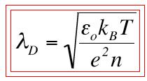
31 σ x,y,z << λ D σ x,y,z >> λ D

32 Continuous Uniform Cylindrical Beam Model I ρ = π R v R J = I π R Gauss s law ε o E ds = Ampere s law ρdv I E r = πε o R v r for r R I 1 E r = πε o v r for r > R Ir B dl = µ o J ds B ϑ = µ o πr for r R I B ϑ = µ o for r > R πr B ϑ = β c E r

33 Lorentz Force F r = e( E r βcb ϑ ) = e( 1 β )E r = ee r γ has only radial component and is a linear function of the transverse coordinate The attractive magnetic force, which becomes significant at high velocities, tends to compensate for the repulsive electric force.

34 Bunched Uniform Cylindrical Beam Model L(t) R(t) (0,0) s l v z = βc Longitudinal Space Charge field in the bunch moving frame: ρ = Q πr L E z s,r = 0 ( ) = ρ 4πε o R π L ( l s ) rdrdϕd l & ( l s ) + r 3 / ) '( * + E z ( s,r = 0) = ρ % ε 0 &' ( ) R + ( L s ) R + s + s L ( )*

35 Radial Space Charge field in the bunch moving frame by series representation of axisymmetric field: $ E r (r, s) ρ & % ε 0 s ' E z (0, s) ) r ( + [ ] r E r (r, s ) = ρ ε 0 % ' &' ( L s ) R + ( L + s ) s R + s ( * )* r

36 Lorentz Transformation back to the Lab frame E z = E z E r = γ E r L = γl ρ = ρ γ s = γs E z (0, s) = ρ " R +γ (L s) R +γ s +γ s L γ ε #$ 0 ( ) % &' E r (r,s) = γρ & ( (L s) ε 0 ( + ' R + γ (L s) s R + γ s ) + r + * It is still a linear field with r but with a longitudinal correlation s

37 E z (0,s,γ ) = I πγε 0 R βc h s,γ ( ) E r (r,s,γ ) = Ir πε 0 R βc g s,γ ( ) γ= 1 γ = 5 γ = 10 F r = ee r γ = eir πγ ε 0 R βc g s,γ ( ) R s (t) L(t) Δt

38 The Laminar beam

39 Trace space of an ideal laminar beam " x $ # x! = dx dz = p x $ % p z p x << p z X Paraxial approx. X

40 Trace space of a laminar beam X X

41 Trace space of non laminar beam X X

42 Geometric emittance: Ellipse equation: ε g γx + αx x $ + β x $ = ε g Twiss parameters: βγ α = 1! Ellipse area: A = πε g β = α

43

44 rms emittance σ x' x σ x ε rms + + f x,! x ( x )dx d x! =1 f! x, x! rms beam envelope: + + σ x = x = x f ( x, x &)dxd x & Define rms emittance: ( ) = 0 γx + αx $ x + β $ x = ε rms such that: σ x = x = βε rms σ x' = x! = γε rms Since: α = β $ β = x ε rms it follows: α = 1 ε rms d dz x = x x % ε rms = σ xx' ε rms

45 σ x = x = βε rms σ x' = x ' = γε rms σ xx' = x x! = αε rms It holds also the relation: γβ α = 1 Substituting α,β,γ we get σ x' σ x " σ xx' $ ε rms ε rms # ε rms % ' & =1 We end up with the definition of rms emittance in terms of the second moments of the distribution: ε rms = ( x ) σ x σ x' σ xx' = x x" x "

46 What does rms emittance tell us about trace space distributions under linear or non-linear forces acting on the beam? x ε rms = x x # x x # x a a a x a x Assuming a generic x, x " correlation of the type: x! = Cx n When n = 1 ==> ε rms = 0 ε rms = C ( x x n x n+1 ) When n = 1 ==> ε rms = 0

47 Envelope Equation without Acceleration Now take the derivatives: dσ x dz = d dz d σ x dz = d dz x = 1 σ x σ xx' = 1 dσ xx' σ x σ x dz d dz x = 1 x x! σ x σ xx' σ = 1 x ' 3 x σ x = σ xx' σ x ( x x!! ) σ xx' σ x 3 = σ x' + x x!! σ x σ xx' 3 σ x And simplify: σ!! x = σ xσ x' σ xx' x x!! 3 σ x σ x = ε rms σ + x x!! 3 x σ x We obtain the rms envelope equation in which the rms emittance enters as defocusing pressure like term. σ!! x x x!! σ x = ε rms 3 σ x

48 σ!! x x x!! σ x = ε rms σ x 3 Assuming that each particle is subject only to a linear focusing force, without acceleration: x!! + k x x = 0 take the average over the entire particle ensemble σ x " + k x σ x = ε rms σ x 3 x x!! = k x x We obtain the rms envelope equation with a linear focusing force in which the rms emittance enters as defocusing pressure like term.

49 Bunched Uniform Cylindrical Beam Model E z (0,s,γ ) = I πγε 0 R βc h s,γ ( ) E r (r,s,γ ) = Ir πε 0 R βc g s,γ ( ) γ= 1 γ = 5 γ = 10 R s (t) L(t) Δt

50 Lorentz Force F r = e( E r βcb ϑ ) = e( 1 β )E r = ee r γ is a linear function of the transverse coordinate dp r dt = F r = ee r γ = eir πγ ε 0 R βc g s,γ ( ) The attractive magnetic force, which becomes significant at high velocities, tends to compensate for the repulsive electric force. Therefore space charge defocusing is primarily a non-relativistic effect. F x = eix πγ ε 0 σ x βc g s,γ ( )

51 Envelope Equation with Space Charge Single particle transverse motion: dp x dt d dt x!! = = F x p x = p x! = βγm o c x! ( p x! ) = βc d dz p x! F x βcp ( ) = F x F x = eix πγ ε 0 σ x βc g s,γ ( ) x!! = k sc s,γ ( ) σ x x

52 Now we can calculate the term x x " that enters in the envelope equation σ x " = ε rms 3 σ x x " x σ x!! x = k sc σ x x x x!! = k sc σ x x =k sc Including all the other terms the envelope equation reads: σ!! x + k σ x = Space Charge De-focusing Force ε n ( βγ) σ + k sc 3 x σ x Emittance Pressure External Focusing Forces Laminarity Parameter: ( ρ = βγ ) k sc σ x ε n

53 The beam undergoes two regimes along the accelerator σ x " + k σ x = ε n ( βγ) σ + k sc 3 x σ x ρ>>1 Laminar Beam σ x " + k σ x = ε n ( βγ) σ + k sc 3 x σ x ρ<<1 Thermal Beam

54 Laminarity parameter ρ = Iσ γi A ε Iσ q n γi A ε = 4I n γ ' I A ε n γ Transition Energy (ρ=1) γ tr = I # γ I A ε n ρ I=4 ka ε th = 0.6 µm E acc = 5 MV/m I=1 ka Potential space charge emittance growth I=100 A ρ = 1

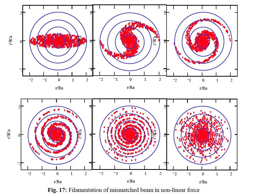
55 Space charge induced emihance oscilla*ons in a laminar beam

56 Neutral Plasma Surface charge density Surface electric field Restoring force Plasma frequency Plasma oscillations

57 Neutral Plasma Oscillations Instabilities EM Wave propagation Single Component Cold Relativistic Plasma Magnetic focusing Magnetic focusing

58 ( ) σ " + k s σ = k sc s,γ σ Equilibrium solution: ( ) = k sc( s,γ ) σ eq s,γ k s Single Component Relativistic Plasma k s = qb mcβγ Small perturbation: σ( ζ ) = σ eq ( s) +δσ ( s) δ σ # s ( ) + k s δσ ( s) = 0 δσ ( s) = δσ o ( s)cos( k s z) Perturbed trajectories oscillate around the equilibrium with the same frequency but with different amplitudes: σ( s) = σ eq ( s) +δσ o ( s)cos( k s z)

59 Emittance Oscillations are driven by space charge differential defocusing in core and tails of the beam p x Projected Phase Space x Slice Phase Spaces

60 Perturbed trajectories oscillate around the equilibrium with the same frequency but with different amplitudes X X

61 Envelope oscillations drive Emittance oscillations σ(z) ε(z) ε rms = ( x ) sin k s z σ x σ x' σ xx' = x x % x % ( )

62 References: [10] C. Prior, Special Relativity, CAS Proceedings, CERN [11] W. Greiner CLASSICAL MECHANICS - Point Particles and Relativity, Springer