Orthogonal Frequency Division Multiplexing (OFDM) in Long Term Evolution (LTE)

Transcript

1 Orthogonal Frequency Division Multiplexing (OFDM) in Long Term Evolution (LTE) Καθηγητής Γεώργιος Ευθύµογλου

2 Wireless channel models There are two distinct fading models for the wireless channel 1. 1 path 0 multipath delay frequency flat fading channel 2. Multiple paths frequency selective fading channel 2

3 Received Signal Multipath delays occur as a transmitted signal is reflected by objects in the environment between a transmitter and a receiver. 3

4 Received Signal in Single Carrier systems Multipath delays causes intersymbol interference (ISI) in the received symbols, because time dispersion occurs where the energy from one symbol spills over into other symbols. h0 x s1 s2 s3 s4 s5 s6 s7 h1 x s1 s2 s3 s4 s5 s6 s7 h2 x s1 s2 s3 s4 s5 s6 s7 Example: delay spread = 7 symbol times Received signal is given by linear convolution of transmit signals with the impulse response of the channel. 4

5 Received signal Frequency Flat fading channel (narrowband systems) ( ) r n = h( n) s( n) + w( n) ( ) ( n) = + ( ) ( ) jθ a n e s n w n Frequency selective channel (wideband systems) ( ) r n = h( n)* s( n) + w( n) L 1 l= 0 ( ) ( ) ( ) = + h l s n l w n Each multipath component is typically associated with different time delay and attenuation, the shortest of which is the LOS path. 5

6 OFDM using N orthogonal subcarriers 1 TOFDM = = N T f k Fs fk = k f = N s N 1 N 1 k Fs j 2 t j 2π fkt N x(t) = X ( k) e = X ( k) e π k= 0 k= 0 ιαµόρφωση OFDM: Όλοι οι υπο-δίαυλοι, ταυτόχρονα, χρησιµοποιούνται από τον ίδιο χρήστη. Κάθε υπο-δίαυλος «κουβαλάει» ένα σύµβολο διαµόρφωσης. 6

7 OFDM vs Single Carrier OFDM: κάθε υπο-δίαυλος «κουβαλάει» ένα σύμβολο διαμόρφωσης Single Carrier: κάθε σύμβολο καταλαμβάνει όλο το φάσμα για μικρό χρόνο 7

8 Πλεονεκτήµατα του OFDM vs Single Carrier 1) Η διάρκεια εκποµπής κάθε συµβόλου διαµόρφωσης αυξάνεται Ν φορές. Εποµένως, οι πολλαπλές διαδροµές που φτάνουν κατά τη διάρκεια ενός συµβόλου διαµόρφωσης θα επηρεάζουν µόνο ένα µικρό µέρος του συµβόλου. 2) Η επίδραση του πολυδιαδροµικού καναλιού µπορεί να «εξουδετερωθεί»µε τη χρήση του κυκλικού προθέµατος. 3) Έχουµε frequency diversity γιατί κάθε σύµβολο πολλαπλασιάζεται µε διαφορετικό συντελεστή καναλιού. 4) Ένας χρήστης δύναται να εκπέµψει µέρος του φάσµατος εκποµπής, ενεργοποιώντας συγκεκριµένους subcarriers. 8

9 OFDM example Using single carrier with data rate of 10 Mbps with QPSK modulation (2 bits per symbol, BW=5MHz) gives a symbol rate Rs = 5 Msymbols/sec or symbol time Ts = 1/(5M sym/sec) = 0.2 μseconds. With a bandwidth of 5 MHz, if we have an OFDM system with 1000 carriers, the OFDM symbol time is T OFDM =1/Δf=1/(5MHz/1000)=200μseconds. = 1/(5MHz/1000) = At the speed of light, an object in an urban environment (typically 1 Kmaway)generatesadelayof6.6μsec. This reflected signal would be completely out of sync with the direct signal and will affect 6.6/0.2 = 33 symbols with single carrier system. However, for OFDM, the delay of 6.6 μseconds is only 1/30th of the OFDMsymboldurationT OFDM =200μseconds.

10 CALCULATING THE NUMBER OF SUBCARRIERS BASED ON MULTIPATH DELAY SPREAD The number of subcarriers can be calculated for a given bandwidth based on the delay spread of the channel. As an example, if the delay spread is 20 µseconds, in order that the subcarriers have flat fading, the OFDM symbol duration should be at least 10 times the delay spread or T OFDM =200µseconds. The OFDM symbol duration is then 200 µseconds (including the guard band) and the bandwidth of each subcarrier is 1/200 = 5 KHz. If the channel bandwidth is 1 MHz, 200 subcarriers can be used for OFDM operation.

11 CALCULATING THE NUMBER OF SUBCARRIERS BASED ON MULTIPATH DELAY SPREAD Περιορισμοί στο Φασματικό Πεδίο Το μοντέλο καναλιού Vehicular Β ITU-R, παρουσιάζει τιμές καθυστέρησης έως 20 μsec, για κινητά περιβάλλοντα. Ο σχεδιασμός της απόστασης Δf των υποφερόντων απαιτεί flat fading για κάθε υπο-φέρον ακόμα και για τις χειρότερες τιμές καθυστέρησης των 20 μsec. Το coherence bandwidth, δηλαδή το εύρος ζώνης που παρουσιάζει την ίδια διάλειψη, υπολογίζεται να είναι περίπου 10KHz: 1 1 B c 10KHz 5 τ = 5 20µs = max Περιορισμοί στο Χρονικό πεδίο Η μέγιστη ταχύτητα για την υποστήριξη κινητικότητας είναι 125Km/hr. Η μέγιστη μετατόπιση Doppler στα 3.5GHz είναι: f D ν 35 m / s = = = 408 Hz λ 0.086m Χρησιμοποιώντας ένα εύρος ζώνης υπoφέροντος ίσο με 10KHz, η ισχύς Διακαναλικής Παρεμβολής (InterCarrier Interference) που αντιστοιχεί στην παραπάνω μετατόπιση Doppler φαίνεται ότι περιορίζεται στο -27dB.

12 Εφαρµογή Θέλουμε να σχεδιάσουμε ένα OFDM σύστημα με f c =2.5GHz, BW < 20MHz που να μεταφέρει δεδομένα με ρυθμό R b =10.24Mbpsκαιμερυθμόκωδικοποίησης(FEC)ρ=1/2. H μέγιστη ταχύτητα του δέκτη είναι v max = 216km/h και ο δίαυλοςέχειτ max =8μsec. Θέλουμε επίσης για τη χρήσιμη διάρκεια του OFDM συμβόλουναισχύει5τ max T sym 0.03T coh όπου Coherence time Τ coh του καναλιού είναι η χρονική διάρκεια στην οποία το κανάλι παραμένει σταθερό. 12

13 Εφαρµογή vmax Max. Doppler Shift : fd,max = fc = 500Hz c 1 Coherence Time : Tcoh = 2msec f D,max OFDM Symbol Duration : T = 5 τ = 40µ sec< 0.03 T = 60µ sec max 1 Sub-Carrier Spacing : f = = 25kHz T Cyclic Prefix Duration : T CP OFDM OFDM τ max TCP = 10µ sec coh 13

14 Εφαρµογή Assume Number of Sub-Carriers : N = 512 N fft Rb = Rskρ = k TO FDM + TCP ( ) fft BW = N f = 12.8 MHz, (<20MHz) ρ Rb TOFDM + TCP k = k = 2 bits / symbol QPSK N ρ 6 SINGLE CARRIER : Rs = = symbols / sec max s fft n = τ R 82 R 2 ρ fft Χωρίς OFDM, 82 διαδοχικά σύµβολα QPSK επηρεάζονται από ISI 14

15 Spectrum of OFDM orthogonal carriers IfwetakeanFFTofanOFDMsignalweseethatwheneachcarrier has a peak, all others are zero. This is expected, since the spectrum of each sub-carrier of length T has a zero at multiples of 1/T(peaks of other subcarriers) N=16 Subcarriers of OFDM signal amplitude frequency bins with N*16 resolution 15

16 Spectrum of OFDM orthogonal carriers Bandwidth of multi-carrier signal. Sub carriers Carrying data Data carried by each subcarriers (Sampling Point on Frequency Domain) Summation of all sub carriers Sampling Point on Frequency Domain 16

17 Carriers with duration T sec (1/10) Example: BW = Fs = 20MHz and N=128 In the 20MHz spectrum, there are 128 narrowband sub-carriers. The duration of each subcarrier is N 128 T = NTs = = = 6.4µ sec 6 F s The frequency separation between them is fixed at 1 1 Fs 20MHz = = = = KHz T NT N 128 The 128 subcarrier frequencies are s { 0, , 2* , (127)*156.25} KHz 17

18 Carriers with duration T sec (2/10) Assume a complex sinusoid j t e π Its spectrum is given in the next slide and is obtained by ( f )*sinc( f T) δ with duration T=100 µsec The shape of the function sinc(f T) has zeros at frequencies: = 0, 10, 20, 190, 210, 220 KHz, that is at multiplies of 1 1 f = = = 10KHz 4 T 10 sec Therefore, if we have a BW=Fs=1MHz, we can have frequency spacing between subcarriers f = 10KHz, that is, we can have BW 1000KHz N = 100 f = 10KHz = 18

19 Carriers with duration T sec (3/10) Observe that frequency nulls exist at all frequencies given by k /, { 0,1,2,..., 19,21,22,...99 } 5 { 0,1,2,..., 19,21,22,...99 } 10 Hz f = k T k= = spectrum of 200KHz with duration T=100µsec ans sampled with Fs=1MHz Amplitude Frequency, Hz x

20 Carriers with duration T sec (4/10) Spectrum of a single subcarrier with time duration Tu ( π f T ) sin u = π f Tu 2 ( sinc( f Tu) ) 2 20

21 Carriers with duration T sec (5/10) Example: BW=Fs=20MHz and Δf = KHz 1 1 The duration of each subcarrier is T = = = 3 f µ sec The number of subcarriers are given by N = Fs 20MHz 128 f = MHz = The 128 subcarrier frequencies are { 0, ,..., } KHz 21

22 Carriers with duration T sec (6/10) The N subcarrier frequencies can be written as k k k Fs fk = = =, k = 0,1,..., N 1 T NT N s The discrete time signal is given by k k n k n sk = exp j 2 π nts = exp j 2 π = exp j 2 π, k = 0,1,..., N 1 T NTs F s N n= 0,1,..., N 1 Theory: Two sinusoids that occupy time T will be orthogonal 1/T iff their frequency separation f is a multiple of!! Result:All N subcarriers s k with duration N samples are orthogonal 22

23 Carriers with duration T sec (7/10) For example, assume Fs = 16 and N=16 (T=N/Fs=1sec) The subcarrier frequencies are The spectrum of subcarrier f 10 is sinc ( f T) *δ( f f ) 10 k k Fs k16 f = k k ( Hz), k 0,1,...,15 T = N = 16 = = spectrum of 1 subcarrier with N samples Sinc centered around f Notice that sidelobes have nulls at the frequencies k k Fs k16 f = k k Hz k k T = N = 16 = = amplitude ( ), 0,1,...,15, frequency bin 23

24 Carriers with duration T sec (8/10) Spectrum of 16 samples of frequency 10 Hz with sampling freq. 16Hz Matlab code for previous plot: clear Fs=16; f0=10; N=16; x1t = exp(j*2*pi*f0*[0:n-1]/fs); % exp(j 2 π f0 t) with t = n Ts x1f = fft(x1t, N*16); % 16 x resolution in frequency domain figure (1) plot([0:n*16-1]/16, x1f) xlabel('frequency bin') ylabel('amplitude') title('spectrum of 1 subcarrier with N samples') 24

25 Carriers with duration T sec (9/10) When two sinusoids occupy time T=NTs, then if their frequency separation is then the sinusoids will be orthogonal (peak of 1 carrier happens at k k kf s = =, k integer T NT N spectrum of 2 subcarriers with N samples 18 s a null frequency of the other). amplitude frequency bin 25

26 Carriers of limited duration (10/10) Consider 16 samples of 2 frequencies 5 and 10 Hz with sampling freq. 16Hz. Their frequency separation is 5 Hz = k*fs/n = k*16/16 for k=5; clear Fs=16; f0=10; f1 = 5; N=16; x1t = exp(j*2*pi*f0*[0:n-1]/fs) + exp(j*2*pi*f1*[0:n-1]/fs) ; x1f = fft(x1t, N*16); % 16 x resolution in frequency domain figure (1) plot([0:n*16-1]/16, x1f) xlabel('frequency bin') ylabel('amplitude') title('spectrum of 2 subcarriers with N samples') 26

27 Generation of OFDM sub-carriers using IDFT (1/3) Example: generate the 5 th (k=5) subcarrier with frequency 5* MHzandamplitude0.5(BW=Fs=20MHzand N=128) Input signal X(k) is sampled with Fs and goes through a serial to parallel conversion. Inputvector X=[zeros(1,5),0.5,zeros(1,128-6)] T atinputofidftof length 128. X (0) = 0 X (5) = 0.5 X ( N 1) = 0... IFFT(X,N) 1 sk ( n) = 0.5exp j2π 5* n 20 5n = 0.5exp j2 π, n= 0,1,..., N

28 Generation of OFDM sub-carriers using IDFT (2/3) All complex sinusoids k k n k n sk = exp j2π nts = exp j2π = exp j2 π, k = 0,1,..., N 1 T NTs F s N transmitted for duration N*Ts=T will be orthogonal, since they differ in frequency between them by integer multiple of(1/t). Therefore, we can use each frequency signal to transmit one symbol X(k) (symbol is BPSK or QPSK or 16-QAM, etc). Then we can addtheminparallelfordurationt(nsamples)andtransmitthem N 1 kn x( n) = X ( k)exp j2 π, n= 0,1,..., N 1 (A) k= 0 N However, eq. (A) is the IDFT of vector X (symbol vector) s k 28

29 Generation of OFDM sub-carriers using IDFT (3/3) We can use each frequency f k =k*f s /N, k=0,1,,n-1 to transmit one symbol X(k) (symbol is BPSK or QPSK or 16-QAM, etc). Then we can add them in parallel for duration T OFDM =N*T s (N samples) and transmit N symbolsasablock.allthishappenswith1ifftdsp: Serial Symbol Source (BPSK, QPSK, 16-QAM, 64-QAM) N 1 kn x ( n ) = X ( k )exp j 2 π, n = 0,1,..., N 1 k= 0 N Serial To Parallel IFFT Parallel To Serial Cyclic Prefix Channel 29

30 Plotting the OFDM Spectrum (1/6) fsmhz = 20; fcmhz = ; N = 128; % sampling frequency % signal frequency % fft size % generating the time domain signal x1t = exp(j*2*pi*fcmhz*[0:n-1]/fsmhz); x1f = fft(x1t,n); % 128 point FFT figure; plot([-n/2:n/2-1]*fsmhz/n, fftshift(abs(x1f))) ; % sub-carriers from [-64:63] xlabel('frequency, MHz') ylabel('amplitude') title('frequency response of complex sinusoidal signal'); To fftshiftµετατοπίζει τις τιµές από το [Fs/2, Fs) [-Fs/2, 0), ώστε η µηδενική συχνότητα να είναι στο µέσο του φάσµατος. 30

31 Plotting the OFDM Spectrum (2/6) With an N =128 point fft() and sampling frequency of f s, the observable spectrum from is split to sub-carriers. However, the signal at the output of fft( ) is from As the frequencies from get aliased to the operator fftshift() is used when plotting the spectrum. 31

32 Plotting the OFDM Spectrum (3/6) Για ένα σύστηµα OFDM µε Ν=128 και συχνότητα δειγµατοληψίας F s βρείτε µε ποια συχνότητα βασικής ζώνης είναι ισοδύναµη η συχνότητα f 70 = 70 (F s /128), η οποία είναι µεγαλύτερη από την F s / 2.Αποδείξτετοµετηχρήσητουλογισµικού Matlab. Λύση Η παραπάνω συχνότητα, όταν δειγµατοληπτηθεί µε συχνότητα δειγµατοληψίας θα εµφανιστεί στη βασική ζώνη, διάστηµα [-F s /2, F s /2) [-64:63), ως η f -58 = -58 (F s /128), όπως αποδεικνύει η παρακάτω µαθηµατική σχέση: j π nt s s 128 j j π n π π 128 n j π n T 128 e = e = e = e 32

33 Plotting the OFDM Spectrum (4/6) clear; N=128; k1=70; k2=-58; n = [0:N-1]; x1 = exp(j*2*pi*k1*n/n); x2 = exp(j*2*pi*k2*n/n); plot(n, real(x1), 'bo-') hold on plot(n, real(x2), 'rx-') xlabel('sample number, n') ylabel('amplitude') 33

34 Plotting the OFDM Spectrum (5/6) In the example above, with a sampling frequency of 20MHz, the spectrum from [-10MHz, +10MHz) is divided into 128 sub-carriers with spaced apart by 20MHz/128 = kHz. The generated signal x1t of frequency MHz corresponds to the information on the 10th sub-carrier (starting from 0), which can also be generated from the IFFT as follows: Note the position of 1 in the input to the IDFT: x2f = [0 zeros(1,9) 1 zeros(1,n-10-1)]; x2t = N*ifft(x2F); % time domain signal using ifft() Ή ισοδύναµα x2f = [zeros(1,n/2) 0 zeros(1,9) 1 zeros(1,n/2-10-1)]; x2t = N*ifft(fftshift(x2F)); % time domain signal using ifft() To fftshiftµετατοπίζει τις τιµές από το αριστερό µισό στο δεξιό µισό. 34

35 Plotting the OFDM Spectrum (6/6) fsmhz = 20; % sampling frequency fcmhz = ; % signal frequency N = 128; % fft size % generating the time domain signal x1t = exp(j*2*pi*fcmhz*[0:n-1]/fsmhz); x2f = [zeros(1,n/2) 0 zeros(1,9) 1 zeros(1,n/2-10-1)]; % valid frequency on 10th subcarrier, rest all zeros x2t = N*ifft(fftshift(x2F)); % time domain signal using ifft() % comparing the signals diff = x2t - x1t; err = diff* diff'/length(diff) % this will give 0 35

36 Generation of OFDM symbol for WiFi Spectrum representation of OFDM symbol in a, N= FFT Size(=64) sub carries Guard band 26 sub carriers carrying Bits 26 sub carriers carrying Bits 6 sub carries Guard band DC No Subcarrier 36

37 Generation of OFDM symbol for WiFi Assume BPSK symbols to be sent. [1,-1,-1,1,,-1,1,1,-1,,1,1,1,-1] (52 bits) subcarrierindex_data = [-26:-1 1:26]; [1,-1,-1,1,,-1,1,1,-1,,1,1,1,-1] 37

38 Generation of OFDM symbol for WiFi IFFT transforms signal to time domain. frequency ModSequenceForSubCarriers = fftshift(modsequenceforsubcarriers); Shift Rotate frequency 0 frequency frequency ModSequenceInTimeDomain = ifft(modsequenceforsubcarriers,totalnumber OfSubCarrier); IFFT frequency time 38

39 OFDM spectrum Φάσµα εκποµπής για σήµα OFDM µε Ν=64, Fs = 20MHz 39

40 OFDM transmitter with encoder and interleaver Block diagram of OFDM transmitter 40

41 Interleaver Most error-correcting codes, both block codes and convolutional codes, cannot correct many errors if they occur close together. Typically, the codes can correct between one and five errors in blocks of data of perhaps 10 to 100 bits. In practice, errors often do not occur like this at all: in many cases we get bursts of tens or even hundreds of errors occurring very infrequently, and no errors for the rest of the time. A technique which can be employed to allow error-correcting codes to protect against bursts is interleaving. Figure below shows how interleaving might be used in association with (7,4) Hamming code so that it is able to correct up to four consecutive errors. Four consecutive code words are interleaved by writing the words into a 4 7 matrix of memory locations row by row, and reading out column by column. 41

42 Interleaver example consecutive code words are interleaved by writing the words into a 4 7 matrix of memory locations row by row, and reading out column by column. 42

43 De-interleaver example The interleaving is undone at the receiver by writing the received bits into a matrix column by column, and reading out row by row. un-interleaving has the effect of spreading out the errors so that each of the four code words contains only a single error, which can be corrected. 43

44 Burst errors look like random errors 44

45 Burst errors look like random errors The interleaving is undone at the receiver by writing the received bits into a matrix column by column, and reading out row by row. If we now have a burst of four errors on the channel, so that four consecutive bits in the data arriving at the receiver are errored, the un-interleaving has the effect of spreading out the errors so that each of the four code words contains only a single error, which can be corrected. The interleaving takes place after the coding at the transmitter, and the un-interleaving takes place before the decoding at the receiver. That is, the sequence is coding interleaving channel de-interleaving decoding. 45

46 OFDM transmitter with encoder and interleaver Block diagram of a/g transceiver architecture (Coded OFDM) The sequence of interleaved bits is mapped into a sequence of modulation symbols, e.g., 16-QAM. Therefore, 4 consecutive coded bits at the encoder output will be separated and each coded bit will combine with 3 other bits and will be sent with a different modulation symbol (e.g., 16-QAM), that is, it will be sent with a different subcarrier. 46

47 OFDM transmitter with encoder and interleaver Therefore, at the receiver side, after the Frequency deinterleaver, the probability of 4 consecutive bits are in error is small. In order for 4 consecutive bits to be in error, 4 16QAM symbols with different fading must be wrongly detected. The probability of this to happen is small. So the error bits at the Decoder input will not be consecutive but random. This way the decoder will be able to find the correct valid codeword from the received bits and provide the correct info bits. 47

48 Coded OFDM Problem solution 48

49 Frequency selective channel Multipath propagation results in frequency selective fading. OFDM solution to maintain subcarrier orthogonality is Cyclic Prefix 49

50 OFDM in time domain Transmitted signal is OFDM (block Transmission) Data symbols c k 50

51 Cyclic Prefix (1/5) Το cyclic prefixτου [ ] { } x n ορίζεται ως x[ N M],..., x[ N 1] δηλαδή αποτελείται από τις τελευταίες M τιµές του x n. Για κάθε ακολουθία εκποµπής x n µήκους Ν, αυτά τα Mδείγµατα µπαίνουν στην αρχή της ακολουθίας εκποµπής. Αυτό δηµιουργεί [ ] [ ] µία νέα ακολουθία x n µήκους Ν+M: [ ] [ ] = [ ],..., [ 1 ], [ 0 ],..., [ 1] x n x N M x N x x N x[n-m] x[n-m+1] x[n-1] x[0]x[1] x[2]... x[n-m-1] x[n-m] x[n-m+1] x[n-1] 51

52 Cyclic Prefix (2/5) OFDM symbol with cyclic prefix Total OFDM symbol time is T u + T g SNR loss 1 Tguard T 4 SNR 1dB loss T = 10 log 1 T useful guard total 52

53 Cyclic Prefix (3/5) Έστω ότι το x [ n] είναι είσοδος στο κανάλι πολλαπλών διακριτών διαδροµών (ισοδύναµο µε ένα FIR φίλτρο). Η έξοδος θα είναι: [ ] = [ ]* [ ] y n x n h n L [ ] [ ] = h k x n k k= 0 k= 0 [ ] [ ] [ ] h[ n] όπου η τρίτη ισότητα ισχύει για M>Lεπειδή για L = h k x n k = x n N N [ ] [ ] 0 k M 1, x n k = x n k for 0 n N 1. N 53

54 Cyclic Prefix (4/5) Εποµένως µε την προσθήκη του cyclic prefixστα Ν δείγµατα εκποµπής, η γραµµικήσυνέλιξη του σήµατος εκποµπής µε το κανάλι, που δίνει το y[n] για 0 n N 1, ισούται µε την κυκλικήσυνέλιξη του αρχικού σήµατος µε το κανάλι. Παίρνοντας εποµένως στο δέκτη το DFTτου y[n] (χωρίς θόρυβο) έχουµε: { N } [ ] [ ] [ ] [ ] [ ] [ ] Y k = DFT y n = x n h n = X k H k, 0 k N 1 N και εποµένως, αν γνωρίζουµε το DFT{h}, τα σύµβολα εκποµπής µπορούν να βρεθούν στο δέκτη µε µία απλή διαίρεση: { vector y } { vector h } DFT N { } vector{ X} = DFT { } N 54

55 Cyclic Prefix (5/5) X x y Y CP x h (CIR) x= IFFT { X} CP y= x h= x h { } { } { } { } Y= FFT y = FFT x h = FFT x FFT h = X H : Convolution, : CircularConvolution : Dot product Άρα, γνωρίζοντας τα Υ, Η, το Χ βρίσκεται µε απλή διαίρεση 55

56 Μετάδοση και λήψη OFDM µε κυκλικό πρόθεµα Στο OFDM αντί να στείλουµε κάποια σύµβολα διαµόρφωσης (π.χ. +1 bit 1και -1 bit 0)στέλνουµετηνέξοδοτου ifft Νσυµβόλων εκποµπής. Π.χ. ifft([ ], 4) ans = Επίσης, επειδή το σήµα εκπέµπεται σε ένα πολυδιαδροµικό κανάλι, το οποίο ενεργεί σαν φίλτρο, π.χ. h = [0.7, -0.3]. Προσθέτουµε το κυκλικό πρόθεµα στο υπάρχων σήµα εκποµπής. Ο αριθµός αυτών των δειγµάτων πρέπει να είναι µεγαλύτερος ή τουλάχιστον ίσος µε το µήκος του πολυδιαδροµικού καναλιού (φίλτρου). Εστω ότι επιλέγουµε µήκος κυκλικού προθέµατος 3. 56

57 Μετάδοση και λήψη OFDM µε κυκλικό πρόθεµα Το λαµβανόµενο σήµα στο δέκτη θα είναι: y = conv([ ], [ ]) y = Στο δέκτη, πετάµε τα πρώτα 3 δείγµατα (αντιστοιχούν στο κυκλικό πρόθεµα)και ταεπόµεναν(εδών=4)ταβάζουµεείσοδοσεένα DFT (fft in Matlab) και διαιρούµε µε την απόκριση συχνότητας του καναλιού υπολογισµένη σε Ν συχνότητες: x = fft([ ],4)./ fft([ ], 4) x =

58 OFDM in frequency domain Each data symbol c k is modulated by a subcarrier 58

59 SubCarriers with duration T OFDM sec The N subcarrier frequencies can be written as k k k Fs fk = = =, k = 0,1,..., N 1 T NT N OFDM s The discrete time signal of k-th subcarrier is given by k k n k n sk = exp j2π nts = exp j2π = exp j2 π, n= 0,1,..., N 1 TOFDM NTs Fs N Theory: Two sinusoids that occupy time duration N*Ts=T OFDM will be orthogonal iff their frequency separation f is : k f =, k= 1,2,... T OFDM Result:All N subcarriers s k with duration N samples are orthogonal 59

60 SubCarriers with duration T OFDM sec Example: BW=Fs=20MHz and Δf = KHz 1 1 The duration of each subcarrier is T OFDM = = = 3 f µ sec The number of subcarriers are given by N = Fs 20MHz 128 f = MHz = The 128 subcarrier frequencies are { 0, ,..., } KHz 60

61 Data Rates for OFDM The OFDM symbol duration is defined by the subcarrier spacing. For example, in Fixed WiMAX we have: T OFDM 1 1 = = = 64µ sec f Hz The bit rate achieved by Fixed WiMAX depends on the modulation and coding scheme (MCS) used in each subcarrier and is given by Bit Rate = Nsubcarriers (# bits / modulation symbol) CodingRate T + T OFDM G

62 Estimating data rates For an OFDM system with 192 subcarriers with data, the number of bits carried by an OFDM symbol is 192 *B where B = bits/modulation symbol. Bit Rate = N subcarriers *(# bits / modulation symbol) T G OFDM Numerical example using QPSK and cyclic prefix 8 µsec BitRate 192* 2 = = 72µ sec 5.33 Mbits / sec

63 Spectral efficiency of MCS Assume BW=1 Hz ID Modulation &Coding Scheme Spectral efficiency of MCS (bit/sec/hz) 1 BPSK 1/2 1 x ½ = QPSK 1/2 2 x ½ =1.0 3 QPSK 3/4 2 x ¾ = QAM ½ 4 x ½ = QAM 3/4 4 x 3/4 = QAM 2/3 6 x 2/3 = QAM 3/4 6 x ¾ = 4.5 ( R ) = spectral efficiency of MCS(bit/sec/Hz) ( H ) b MCS BW z 63

64 Estimating data rates in OFDM CAPACITY ANALYSIS OFDM BW efficiency (b/s/hz) 0,69 Modln+coding efficiency (b/s/hz) 0,50 1,00 1,50 2,00 3,00 4,00 4,50 Overall PHY layer efficiency, (b/s/hz) 0,35 0,69 1,04 1,38 2,07 2,76 3,11 User Data Rate, Mbps 1,21 2,42 3,63 4,84 7,26 9,68 10,89 (BW=3.5 MHz) OFDM Bandwidth efficiency' N_fft = Number of OFDM tones 256 N_data = Number of data tone 192 n = Sampling factor 8/7=1,152 Guard band efficiency (192*8/7) /256=0,864 Cyclic prefix guard time factor (Tg/Tb) 0,250 Guard time efficiency 1/(1+0,250)=0,8 OFDM Bandwidth efficiency factor (downlink) 0,864*0,8=0,691 OFDM Bandwidth efficiency factor (uplink) 0,691 64

65 LTE OFDM transmission Consider a time-discrete (sampled) OFDM signal where it is assumed thatthesamplingratefsisamultipleofthesubcarrierspacingδf fs=1/ts=n Δf As Nc Δf can be seen as the nominal bandwidth of the OFDM signal, this implies that N should exceed Nc with a sufficient margin. N/Nc, is the over-sampling of the time-discrete OFDM signal. 65

66 LTE OFDM transmission As an example, for 3GPP LTE the number of subcarriers Nc is approximately 600 in the case of a 10 MHz spectrum allocation. The IFFT size can then, for example, be selected as N = This correspondstoasamplingratefs=n Δf=15.36MHz,where Δf = 15 khz is the LTE subcarrier spacing. The subcarrier spacing Δf. OFDM transmission parameters The number of subcarriers Nc, which, together with the subcarrier spacing, determines the overall transmission bandwidth of the OFDM signal. The cyclic-prefix length TCP. Together with the subcarrier spacing Δf = 1/Tu, the cyclic-prefix length determines the overall OFDM symbol timet=tcp+tuor,equivalently,theofdmsymbolrate. 66

67 LTE OFDM demodulation Recover the modulation symbols 67

68 LTE Downlink: time domain I. Time duration for one frame is 10 ms.this means that we have 100 radio frames per second. II. Sampling frequency for 20MHz bandwidth is 15 KHz * 2048 (IFFT_size) = MHz = Fs III. Sampling time Ts = 1/Fs = 1/(15 KHz * 2048) = 1/ IV MHz = 8 x 3.84 MHz (sampling frequency in UMTS) V. Duration of time slot is 7 OFDM symbols + 7 CPs VI. Number of subframein one frame is 10. VII. Number of slots in one subframeis 2. This means that we have 20 slots in one frame. VIII. Each slot consists of a number of OFDM symbols which can be either 7 (normal cyclic prefix) or 6 (extended cyclic prefix) 68

69 LTE Downlink: time domain Frame structure for LTE in FDD mode (Frame Structure Type 1). 69

70 OFDM transmission There are many advantages to using OFDM in a mobile access system, namely: 1- Long symbol time and guard interval increases robustness to multipath and limits intersymbol interference. 2- Eliminates the need for intra-cell interference cancellation. 3- Allows flexible utilization of frequency spectrum. 4- Increases spectral efficiency due to the orthogonality between sub-carriers. 5- Allows optimization of data rates for all users in a cell by transmitting on the best(i.e. non-faded) subcarriers for each user. 70

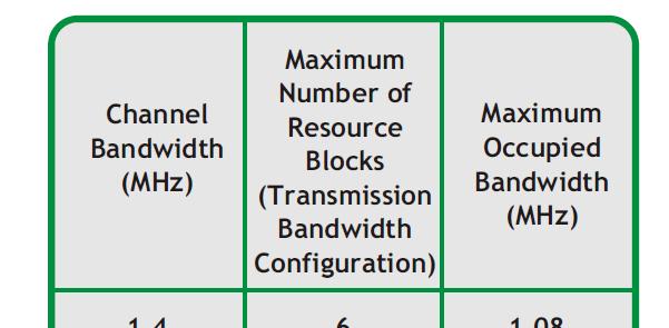
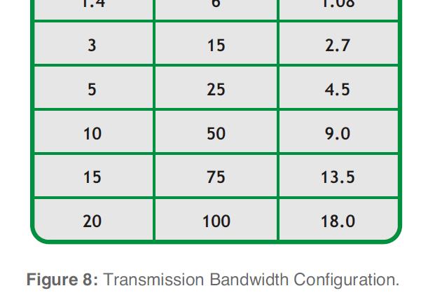
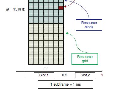
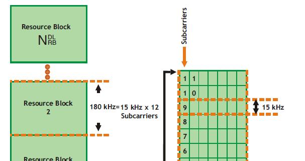
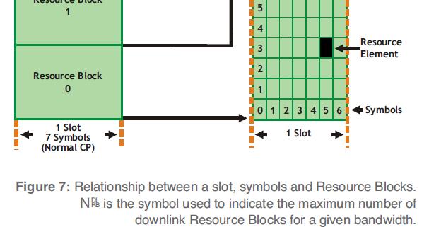
71 LTE Downlink Resources Frequency domain representation of resource block (RB) N RB determines number of subcarriers (12*N RB ) and depends on transmit bandwidth(given below). In the downlink, the DC subcarrier iscounted(+1)butdoesnotusedtosenddata. 71

72 User equipment Concerned with power consumption. Assigned one or more Resource Block (RB) 72

73 Frequency Domain Resources Subcarrier spacing of 15 khz LTE bandwidth is highly flexible 1 MHz to 20 MHz is standard, even more with carrier aggregation 73

74 Resource Block (RB) for downlink RB = 12 subcarriers/slot 74

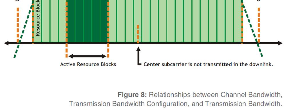
75 Channel bandwidth vs transmission bandwidth 75

76 Transmission bandwidth 76

77 Physical layer parameters for LTE in FDD mode 77

78 78

79 Time Frequency Representation 79

80 LTE Downlink: Resource Block The transmission can be scheduled by Resource Blocks (RB) 1 RB = 12 consecutive sub-carriers, or 180 khz, for the duration of one slot (0.5 ms), that is for (7 OFDM symbols, or 6 for extended CP) A Resource Element (RE) is the smallest defined unit which consists of one OFDM sub-carrier during one OFDM symbol interval. Each Resource Block consists of 12 7 = 84 Resource Elements (RE)in case of normal cyclic prefix (72 for extended CP). Each RE can carry number of bits depending on the modulation employed. For example, using for QPSK: a RB carries 84*2 bits per 0.5 msec. 80

81 LTE Downlink: Resource Block Definition of Resource Blocks and Resource Elements. 1 RB = 12 consecutive sub-carriers, or 180 khz, for the duration of one slot (0.5 ms), that is for (7 OFDM symbols, or 6 for 72 for extended CP) 81

82 LTE Downlink: Resource Block In summary: One frame is 10ms and it consists of 10 sub-frames. OneLTEsubframeis1msandcontains2slots. One slot is 0.5ms in time domain and each 0.5ms assignment can contain N resource blocks [6 < N < 110] depending on the bandwidth allocation and resource availability. One resource block is 0.5ms and contains 12 subcarriers for each OFDM symbol in frequency domain. There are 7 symbols (normal cyclic prefix) per time slot in the timedomainor6symbolsinlongcyclicprefixforlte. LTE Resource element is the smallest unit of resource assignment and its relationship to resource block is shown as below from both a timing and frequency perspective. 82

83 83

84 LTE Downlink: Resource Block Red color for f = 15 KHz. 84

85 LTE: Physical resource blocks (PRBs) or subframes = 1msec In OFDMA, users are allocated a specific number of subcarriers for a predetermined amount of time. Physical resource blocks (PRBs) or Subframe in the LTE specifications equalto 2consecutiveRBs,thatis,12subcarriersfor14OFDMsymbols. 85

86 LTE resource grid 86

87 UE-eNB connection 87

88 LTE Physical Channels Physical channels in the resource grid. 88

89 LTE Physical Channels P-SS: Primary synchronization signal S-SS: secondary synchronization signal PBCH:Physical Broadcast Channel PCFICH: Physical Control Format Indicator Channel PHICH:Physical Hybrid ARQ Indication Channel PDSCH: Physical Downlink Shared Channel PDCCH: Physical Downlink Control Channel PCH: Paging channel RS: Reference Signal, used both in uplink and downlink SRS: Sounding reference signal, used in uplink DMRS: Demodulation Reference Signal PRACH: Physical Random Access Channel used in uplink PUSCH: Physical Uplink Shared Channel PUCCH: Physical Uplink Control Channel 89

90 LTE Physical Channels Resource elements in the resource grid contain six types of data source: User data, Cell Specific Reference (CSR), Downlink Control Information (DCI), PSS, SSS, and BCH. 1. For subframe 0: all the sources of data are present (BCH only in this subframe: it carries Master Information Block, MIB) 2. Forsubframe5:userdata,CSR,DCI,PSS,andSSSarepresent. 3. All other subframes {1, 2, 3, 4, 6, 7, 8, 9}: user data, CSR and DCI symbols are present. 90

91 LTE resource grid 91

92 Radio frame structure (1 antenna port, CFI=2) 92

93 Case 1: Compute Data Rate for 1.4 MHz CFI=2 Given 1.4 MHz of available spectrum, there are 6 Resource Blocks available. There are 3 subframe categories: a) the 1 st one, b) the 5t one c)therest8subframes Thefirst2OFDMsymbolsofeachsubframeisusedforControl Signalling. The6centralRBsinthe1 st subframecontainpbch,pss/sss. Referencesignalsoccupy8REsineachRB. Let s calculate the amount of data and control block for each kind of subframe in 1 RB (12 subcarriers for duration 14 OFDM symbols): 93

94 Case 1: Compute Data Rate for 1.4 MHz CFI=2 Subframe(a):CFI+PBCH+PSS/SSS+reference= 2x12+6x12+4=100 control REs (2 OFDM symbols for CFI, 6=2+4 OFDM symbols for synch+pbch) 12x14-100= 68 data resource elements Subframe (b): CFI + PSS/SSS + reference = 2x12+2x12+6= 54 control REs 12x14-54= 114 data resource elements Subframe(c): CFI + reference= 2x12+6=30 control REs 12x14-30= 138 data resource elements

95 Case 1: Compute Data Rate for 1.4 MHz CF1=2 The overhead can be calculated as (control occupies 6 RB/subframe): Total control= (1 subframe a)x(6x100)+(1 subframe b)x(6x54)+(8 subframe c)x(6x30) = Total resource elements=(6x12)x(10x14)=10080 Overhead (CFI=2)= 100 x (2364/10080)=23.45% 2364 resource elements One information symbol can be allocated in each data resource element. The transmission is done by means of 64-QAM with 6 bits per symbol. The peak rate throughput is: Total data=(1 column a)x(6x68)+(1 column b)x(6x114)+(8 columns c)x(6x138) =7716 resource elements Bit rate= (7716 symbols x 6 bits/symbol)/10ms= 4.5 Mbps 95

96 Case 2: LTE Throughput calculation Let us understand peak data rate or LTE throughput calculation with following LTE system configuration: 20MHz channel, 4x4 MIMO configuration. Theoretically, Peak Data rate = No. of REs per subframe x no. of bits per modulation symbol / subframe time = x 6 / 1msec = bits/ 1 msec Data Rate=100.8Mbps For 4x4 MIMO data rate = 403Mbps About 25% of overhead is used here for RS (reference signal), synchronization signals, PDCCH, PBCH. This leads to effective data rate of about 403Mbps x 0.75 = 302Mbps. 96

97 LTE E-UTRAN LTE targets to achieve 100Mbps in the downlink (DL) and 50 Mbps in the uplink(ul) directions with user plane latency less than 5ms due to spectrum flexibility and higher spectral efficiency. These exceptional performance requirements are possible due to Orthogonal Frequency Division Multiplexing (OFDM) and Multiple-Input and Multiple-Output (MIMO) functionality in the radio link at the physical layer. The Evolved UMTS Terrestrial Radio Access Network (E- UTRAN), the very first network node in the evolved packet system (EPS), achieves high data rates, lower control & user plane latency, seamless handovers, and greater cell coverage. 97

98 References 1. 4G LTE/LTE-Advanced for Mobile Broadband, by Erik Dahlman, Stefan Parkvall, and Johan Skold, 2011 Elsevier. 2. LTE in a Nutshell: The Physical Layer, White paper, 2010, Telesystem Innovations. 3. LTE Resource Guide at sampling-frequency-vs-resource-block.html 5. LTE Physical Layer Overview: Subsystems/lte/Content/lte_overview.html 6. LTE tutorial: LTE E-UTRAN and its Access Side Protocols 9. TS V BS Radio Transmission and Reception 98