ECE 222b Applied Electromagnetics Notes Set 4c

Μέγεθος: px

Εμφάνιση ξεκινά από τη σελίδα:

Download "ECE 222b Applied Electromagnetics Notes Set 4c"

Ἀστάρτη Μητσοτάκης
5 χρόνια πριν
Προβολές:

1 ECE 222b Applied Electromgnetics Notes Set 4c Instructor: Prof. Vitliy Lomkin Deprtment of Electricl nd Computer Engineering University of Cliforni, Sn Diego 1

2 Cylindricl Wve Functions (1) Helmoholt eqution: 2 2 ψ + k ψ ψ 1 ψ 1 ψ ψ k ψ φ Seprtion of vribles: ψ( φ,, ) Ρ( Φφ ) ( ) Z( ) dρ 1 dρ 1 dφ 1 dz k Ρ d Ρ d Φ dφ Z d 2 1 dz Z d dz 2 h + 2 hz jh ( ) ( ) + ( ) d Z Ahe Bhe jh 2

3 Cylindricl Wve Functions 1 d Ρ Ρ Φ d d 1 d Ρ d Ρ d Φ dφ Φ 2 2 m 2 Φ dφ 2 d ( k h ) Φ 2 + m Φ ( ) c cos sin 2 m m + dm m dφ Φφ φ φ 2 2 Ρ Ρ d d + + ( k h ) m 2 Ρ d Ρ d d Ρ dρ ( k ) m 2 Ρ d d k k h Dispersion reltion Ρ( ) J ( k ) + by( k ) m m m m 3

4 Cylindricl Wve Functions (3) J Y m m ( k ) : Bessel functions of the first kind ( k ) : Bessel functions of the second kind Specil properties : 1. J ( x) is finite t x m Y ( x) is infinite t x m 2. J ( x) ~ cos x x m Y ( x) ~ sin x x m Generl solution: ψ( φ,, ) [ J ( k ) + by( k )][ c cos mφ+ d sin mφ] m m m m m m jh jh [ Ahe ( ) + Bhe ( ) ] 4

5 Cylindricl Wve Functions (4) J Y m m ( x): Bessel functions of the first kind ( x): Bessel functions of the second kind x x 5

6 Circulr Wveguides (1) TM modes: y sin mφ E EJ m( k ) e cos mφ E ( φ+ 2 π) E ( φ) cos m( φ+ 2 π) cos mφ sin m( φ+ 2 π) sin mφ jk ε, µ Boundry condition: x m,1, 2, E Jm( k) Denote J ( χ ) then k χ m mn mn 6

7 Circulr Wveguides Propgtion constnt: χmn k k k k k k Cutoff wvenumber: First four modes: k cmn χ mn rel k > k img. k < k f cmn χmn 2π µε TM1 TM11 TM21 TM2 7

8 Circulr Wveguides (3) TE modes: y sin mφ H HJ m( k ) e cos mφ H ( φ+ 2 π) H ( φ) cos m( φ+ 2 π) cos mφ sin m( φ+ 2 π) sin mφ m,1, 2, jk x ε, µ Boundry condition: H J ( k) Denote J ( χ ) then k χ m mn mn m 8

9 Circulr Wveguides (4) Propgtion constnt: rel k > k χ mn k k k k k k Cutoff wvenumber: First four modes: k cmn χ mn img. k < k f cmn χ mn 2π µε Dominnt mode TE11 TE21 TE1 TE31 9

10 Circulr Wveguides (5) Wveguides tht cn be nlyed similrly: 1

11 Coxil Wveguide (1) TM modes: sin mφ E [ mjm( k) + by m m( k)] e cos mφ jk y Boundry condition: E E b x J ( k) + by( k) m m m m ε, µ J ( kb) + by( kb) m m m m 2 2 k k k mn Chrcteristic eqution: J ( ky ) ( kb) Y( kj ) ( kb) m m m m 11

12 Coxil Wveguide TE modes: sin mφ H [ mjm( k) + by m m( k)] e cos mφ Boundry condition: m,1, 2, H H b J ( k) + by ( k) m m m m J ( kb) + by ( kb) m m m m Chrcteristic eqution: jk y ε, µ k k k 2 2 mn x J ( ky ) ( kb) Y ( kj ) ( kb) m m m m k mn,, 12

13 Coxil Wveguide (3) The nlysis given bove is crried out bsed on the ssumption tht k. When m nd k, there is specil solution to the eqution: A 1 A k A 2 2 A Specil solution: A Cln e jk E H φ C 1 jk e E E µε φ C 1 jk e H H µ TEM mode 13

14 Circulr Cvity (1) TM modes: sin mφ E EJ m( k ) cos k cos mφ k χmn, kh pπ p,1, 2, h k + k k ω µε y ω TM 1 mn r mnp 2 2 χ pπ + µε h x 14

15 Circulr Cvity TE modes: sin mφ H HJ m( k ) sin k cos mφ k χ, kh pπ p 1, 2, mn h k + k k ω µε y ω TE 1 mn r mnp 2 2 χ pπ + µε h x 15

16 Circulr Dielectric Wveguide (1) y y x ε 1, µ 1 ε 1, µ 1 ε 2, µ 2 ε 2, µ 2 x Rel dielectric wveguide Simplified version for nlysis 16

17 Circulr Dielectric Wveguide Inside the dielectric wveguide: sin mφ E1 AJ 1 m( k1 ) e cos mφ jk y cos mφ H1 BJ 1 m( k1 ) e sin mφ Outside the dielectric wveguide: jk sin mφ E2 AH 2 m ( k2 ) e cos mφ cos mφ H2 BH 2 m ( k2 ) e sin mφ jk jk ε 1, µ 1 ε 2, µ 2 sin mφ E2 AK 2 m( α2 ) e cos mφ cos mφ H2 BK 2 m( α2 ) e sin mφ k jα x 2 2 jk jk 17

18 Circulr Dielectric Wveguide (3) Boundry conditions: E E 1 2 H H 1 2 E E 1φ 2φ H H 1φ 2φ A mk 1 1 µ J ( k ) µ K ( α ) B m 1 m 2 ± ω k1 α 2 k1 Jm( k1) α2 Km( α2) A ε J ( k ) ε K ( α ) mk B + 1 m 1 2 m k1 Jm( k1) α2 Km( α2) ω k1 α2 18

19 Circulr Dielectric Wveguide (4) Chrcteristic eqution: 2 2 mk ( 1 ) ( 2 ) 1 1 µ J m k µ K m α ω k1 α 2 k1 Jm( k1) α2 Km( α2) ε J ( k ) ε K ( α ) k1 Jm( k1) α2 Km( α2) 1 m 1 2 m 2 + k 2 2 ω µε k α ω µε k m 1 m ε r 1 m εr2 m m m m m J () u K () v J () u K () v ( mδ ) u v u J () u v K () v u J () u v K () v 2 u k k ε δ 1 r1 v α k δ ε 2 2 r 2 19

20 Circulr Dielectric Wveguide (5) Axisymmetric modes (m ): 1 J () u 1 K () v εr1 J () u εr2 K () v + + u J () u v K () v u J () u v K () v First solution: εr1 J () u εr2 K () v + u J () u v K () v A1 B 1 E H TM n modes Cutoff: v J ( u ) TM χn kc n ε ε r1 r2 2

21 Circulr Dielectric Wveguide (6) Second solution: 1 J () u 1 K () v + uj () u vk() v A 1 E B H 1 TE modes n Cutoff: v J ( u ) TE χn kc n ε ε r1 r2 Non-xisymmetric modes: m m 1 m ε r 1 m εr2 m m m m m J () u K () v J () u K () v ( mδ ) u v u J () u v K () v u J () u v K () v EH mn modes HE mn modes 21

22 Circulr Dielectric Wveguide (7) Cutoff: HE modes mn uj J m 1 ( u) ( u ) c m c c 2( m 1) m 1 k HE 1n 1 cn 1 χ ε ε r1 r2 EH modes mn uj J m+ 1 ( u) ( u ) c m c c m 1 k EH 1n cn 1 ε χ ε r1 r2 Dominnt mode: HE k c11 HE 11 mode First-order modes: k k ε ε TE TM c1 c1 r1 r2 22

23 Circulr Dielectric Wveguide (8) Dispersion curves for ε r nd ε r k ε ε r1 r2 23

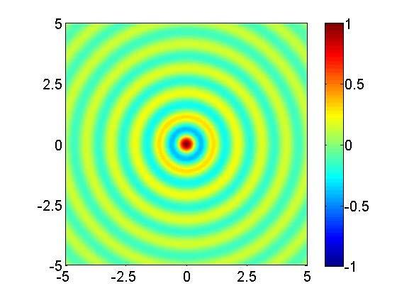
24 Wve Trnsformtion (1) Propgting wve: + jk e cos k + j sin k jk e cos k j sin k Propgting in the - direction Propgting in the + direction Define: H (1) ( k) J ( k) + jy ( k) m m m Propgting in the direction H ( k) J ( k) jy ( k) Propgting in the +direction m m m H, H : (1) m m Hnkel functions of the first nd second kind. 24

25 Wve Trnsformtion Consider plne wve To determine n, jkx e j k x jkcosφ n jnφ n e e e Since 2π 2π jkcosφ jmφ jmφ jnφ n n e e dφ e e dφ 2π 2π j( cos φ+ mφ) m e d j J m k φ 2 π ( ) m m m 2 π j J ( k) 2 π j J ( k) m m m m Therefore jkx e j n J ( ) jn n k e φ n 25

26 Wve Trnsformtion (3) 3 term 21 term 41 term 81 term 161 term 321 term 26

27 Scttering by Circulr Cylinder (1) TM cse: y E E ˆ E ˆ e inc inc jkx Given x Find the scttered field: inc n jn Solution: E E j Jn( k) e φ n sc jn E CH n n ( k) e φ n tot inc sc n jnφ jnφ + n( ) + n n ( ) n n E E E E j J k e C H k e 27

28 Scttering by Circulr Cylinder tot n jn [ n( ) n n ( )] + n E E j J k C H k e φ C n n E j J ( k) H n n ( k) 1.λ 28

29 Scttering by Circulr Cylinder (3) TE cse: H H ˆ H ˆ e inc inc jkx y inc n jn H H j Jn( k) e φ n sc jn H CH n n ( k) e φ n x H H + H tot inc sc From H jωε E E φ 1 H jωε jk jk Eφ H j J k e C H k e tot n jnφ jnφ n( ) + n n ( ) ωε n ωε n 29

30 Scttering by Circulr Cylinder (4) jk E H j J k C H k e φ tot n jn φ [ n( ) n n ( )] + ωε n C n n H j J n( k) H ( k) n 1.λ 3

31 Scttering by Circulr Cylinder (5) TM cse: inc n jn E E j Jn( k) e φ n y ε, µ x int n n d n E E cj ( k) e jnφ ε d, µ d E jωµ H E Hφ Hφ [ j J( k) H ( k)] e inc sc n + n + n n jη n int E H ( ) jn φ cj n n kd e jη d n φ jnφ 31

32 Scttering by Circulr Cylinder (6) Boundry conditions: E + E E inc sc int H + H H inc sc int φ φ φ n n j J n( k) + nh n ( k) cnj n( kd) η j J k H k c J k n n( ) + n n ( ) n n( d ) ηd n µ rj n( k) Jn( kd) εrjn( k) J n( kd) j µ H ( k) J ( k ) ε H ( k) J ( k ) r n n d r n n d c n ( n+ 1) j 2 µ r π k µ H ( k) J ( k ) ε H ( k) J ( k ) r n n d r n n d 32

33 Scttering by Circulr Cylinder (7) TE cse: inc n jn H H j Jn( k) e φ n sc n n n H H H ( k) e jnφ int n n d n H H cj ( k) e jnφ y ε, µ ε d, µ d x H jωε E inc + sc n n + n n n jn E E j H [ j J( k ) H ( k )] e φ φ φ η int E j ( ) jn dh cj n n kd e φ φ η 33 n

34 Scttering by Circulr Cylinder (8) Boundry conditions: H + H H inc sc int E + E E inc sc int φ φ φ n j J n( k) + nh n ( k) cnj n( kd) η j J k H k c J k η n d n( ) + n n ( ) n n( d ) n n ε rj n( k) Jn( kd) µ rjn( k) J n( kd) j ε H ( k) J ( k ) µ H ( k) J ( k ) r n n d r n n d c n ( n+ 1) j 2 ε r π k ε H ( k) J ( k ) µ H ( k) J ( k ) r n n d r n n d 34

35 Scttering by Circulr Cylinder (9) Exmple for TM polrition: 1.λ ε r 4. 35

36 Scttering by Circulr Cylinder (1) Exmple for TE polrition: 1.λ ε r 4. 36

37 Rdition by Line Source (1) Rdition by n infinitely long line current: Method # 1 : ( ) R I y x Method # 2 : 37

38 Rdition by Line Source When 2 2 : A k A + A CH k ( ) Integrted over smll circulr re with vnishing rdius : 38

39 Rdition by Line Source (3) Since A H ( k) C CkH ( k) CkH1 ( k) j2 H1 ( x) x π x A j2 j2c Ck πk π Hence: µ I 4 j A H k ( ) 2 k I ki E H ( k), Hφ H ( k) 4ωε 4j 39

40 Rdition by Line Source (4) 2 H ( k) ~ e x jπ x jx When k >> 1 or >> λ: j jk j E kη I e, Hφ ki e 8πk 8πk For line source locted t : jk µ I ( ) 4 j A H k 4

41 Cylindricl Surfce Current (1) Cylindricl surfce current: Generl solution: x x Field expressions: 2 int jk E (, ) ( ) jn φ J n n ke φ < ωµε n jk E ( φ, ) bh ( k) e jnφ > 2 ext n n ωµε n 41

42 Cylindricl Surfce Current int k H (, ) J( ) jn n n k e φ φ φ < µ n k H (, ) bh ( k ) e jnφ φ φ > ext n n µ n ext int Apply BCs: E (, φ) E (, φ) J k bh k n n( ) n n ( ) (, φ) (, φ) ( φ) ext int Hφ Hφ J s Solutions: 2π µ jnφ J n n( k ) bh n n ( k ) cn cn Js( ) e d 2π k φ φ πk n ch n n ( k ) πk bn cj n n( k ) 2 j 2 j 42

43 Cylindricl Surfce Current (3) Consider specil cse: A line current J s ( φ) Iδφ ( φ ) 2π µ jnφ µ I cn Js( φ) e dφ e 2πk 2πk jnφ Hence, A ( φ, ) µ I Jn( k) Hn ( k ) jn( φ φ ) < e 4 j n Jn( k ) Hn ( k) > Previously, Addition theorem: µ I ( ) 4 j A H k An off-centered cylindricl wve cn be expressed s the superposition of centered cylindricl wves Jn( k) Hn ( k ) jn( φ φ ) < H ( k ) e n Jn( k ) Hn ( k) > 43

44 Cylindricl Surfce Current (4) 3 terms 11 terms 21 terms 31 terms 44

45 Cylindricl Surfce Current (5) Appliction exmple: y Tret this s scttering problem with the scttered field ssumed s Line current sc n n n E (, ) dh ( k ) e jn φ φ σ The incident field is (by the ddition theorem) inc ωµ I E ( φ, ) H ( k ) 4 ωµ I Jn( k) Hn ( k ) jn( φ φ ) < e 4 n Jn( k ) Hn ( k) > x ωµ I J n( k) E d ( ) n H n k e 4 H ( k) n jnφ 45

46 Cylindricl Surfce Current (6) PEC I 1λ 1λ Scttered field Totl field 46

47 Scttering by Conducting Wedge (1) The line current cn be treted s surfce current with A Js ( φ) Iδφ ( φ ) Generl solution: Jν( k) Hν ( k ) ( φ, ) ν Jν( k ) Hν ( k) [ cosνφ + b sin νφ] ν ν < > Line current y α σ x Boundry conditions: E H H φ J φ s E φ α φ 2π + A jπµ < ( φ, ) sin νφ ( α)sin νφ ( α) 2 π α ( ) ( ) > I Jν( k) Hν ( k ) m 1 Jν k Hν k ν mπ (2 π α) 47

48 Scttering by Conducting Wedge Finl solution: E πη J k H k < ( φ, ) sin νφ ( α)sin νφ ( α) 2 π α ( ) ( ) > ki ν( ) ν ( ) m 1 Jν k Hν k H jνπ < ( φ, ) sin νφ ( α)cos νφ ( α) (2 π α) ( ) ( ) > I Jν( k) Hν ( k ) m 1 Jν k Hν k H φ jπ ki J ν( k) Hν ( k ) < ( φ, ) sin νφ ( α)sin νφ ( α) 2 π α m 1 Jν( k ) H ν ( k) > 48

49 Scttering by Conducting Wedge (3) TM polrition TE polrition 49

50 Scttering by Conducting Wedge (4) Close to the edge: k << 1 J ( ) ν ν Line current y H Hφ k << ν 1, when 1 α σ x m 1 nd α < π For : ν π (2 π α) < 1 H, H s φ E, E s φ Edge singulrities Specil cses: (1) α ν 1 2 α π 2 ν 23 5

Σχετικά έγγραφα

ECE Spring Prof. David R. Jackson ECE Dept. Notes 2

ECE Spring Prof. David R. Jackson ECE Dept. Notes 2 ECE 634 Spring 6 Prof. David R. Jackson ECE Dept. Notes Fields in a Source-Free Region Example: Radiation from an aperture y PEC E t x Aperture Assume the following choice of vector potentials: A F = =