Collision Probability Method

Transcript

1 Analy of Stattc Reactor Charactertc nd Semeter of 8 Lecture Note Collon Probablty Method Sept. 8 Prof. Joo Han-gyu Department of Nuclear Engneerng

2 Neutron Tranport Equaton and Soluton Dffculte Boltzmann Neutron Tranport Equaton ˆ v ˆ v v ˆ ˆ ˆ v ˆ ˆ v Ω ϕ ( r, E, Ω + = t ( r, E ϕ( r, E, Ω ( Ω Ω, E E ϕ( r, E, Ω dedω+ χ ( E ψ ( r 4π Ω' E ' Streamng = Net outflow through urface = Ω ( ˆ ˆ x ϕ( x+δx, L, Ω ϕ( x, L, Ω ΔyΔz Term ϕ( x+ Δx, L, Ωˆ ϕ( x, L, Ωˆ ϕ per unt volume lm =Ωx Ω ϕ ˆ n general Δ x Δx x Soluton Dffculte ( re r, N( rtr r, ( r σ ( Tr ( r, E = Strong energy dependence of Xec Angular dependence evere locally Temperature dependence of Xec whch depend on flux through power Practcal Soluton Approache Multgroup Angle dcretzaton(s n or orthogonal expanon (P L Iteraton between flux and T/H feld oluton ϕ( x, L, Ωˆ Ω x x x+ Δx ϕ ( x+ Δx, L, Ωˆ ( x+ Δ x, y+δy, z

3 Three-Step Core Neutronc Calculaton Procedure 3

4 Two Form of Multgroup Tranport Equaton Dfferental (Boltzmann Tranport Equaton Ω ˆ ϕ ( r, Ω ˆ + ( r ϕ ( r, Ω ˆ = Q g tg g g G r ˆ r ˆ ˆ r Q ˆ ˆ g(, Ω = λχψ g + gg (, Ω Ω ϕ g (, Ω dω 4 π g = Integral Tranport Equaton ( otropc ource Q r r R r r ˆΩ R= r [cm] r r ˆ Qg ( r tr r ϕg (, Ω = e dr 4π R R λ t ρ( R dtance n mfp or optcal length φ g ( ρ ( R r e r = Q ( : Scalar Flux g d 4π R f ( φ Integral Equaton 4

5 Scatterng Source n Multgroup Tranport Equaton G r g ˆ gg ϕg Ω g = ˆ ˆ r Q = ( r, Ω Ω (, Ωˆ dωˆ Unnown r ˆ ˆ r = (, (, ˆ ˆ ˆ gg Ω Ω ϕg Ω dω Ω ˆ ˆ ˆ ˆ + (, (, ˆ g g r Ω Ω ϕg r Ω dω Ω Dfferental Scatterng Cro Secton g g :Self catterng, change only drecton Scatterng from other group, condered nown under ource teraton t cheme to multgroup problem ( Ωˆ Ω ˆ = f ( μ g g gg gg where μ =co( θ of the angle θ between Ωˆ and Ωˆ Scatterng ernel 5

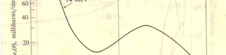
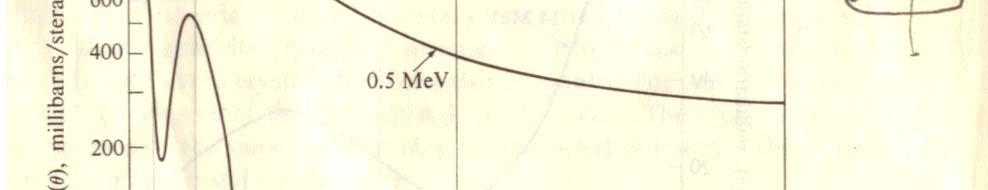
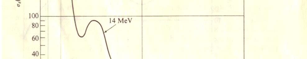
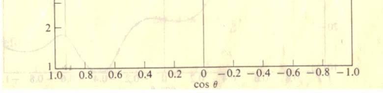
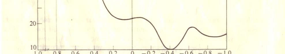
6 Dfferental Scatterng Cro Secton n CMS wave catterng otropc n CMS ( Ql = τ = low energy, lght nucleu C U38 At hgher h energy or for heaver nucle, forward peaed 6

7 Repreentaton of Scatterng Anotropy ˆ dω Dfferental Scatterng Xec Ωˆ ( θ, α ˆ /cm-teradan,e ( θ, E Ed Ω de θ ˆ ˆ : Probablty per unt dtance of travel to =Ω Ω catter nto angle dωˆ around Ωˆ and to de from E Ω ˆ ( θ, α Conderaton of Azmuthal Symmetry ˆΩ n trp ( θ, E Ed Ω= ˆ ( θ, E Ed θ nθ dα π = π θ, E E n θ dθ de θ ( Ωˆ θ 7

8 Legendre Polynomal for Scatterng Antropy Integrate over θ π π ( θ, E E n θ d θ μ = coθ dμ =nθ dθ θ : π θ μ : μ = π ( μ, E Ed μ = ( E E Legendre Expanon of Angular Dependence f ( x = a P( x f ( xp ( xdx = a< PP, > a = < P P > l l l l l l l l= = l, Let f ( μ = π ( μ, E E Momont: π ( μ, ( μ % ( moment ( l al = % ( E E < P, P > l l ( l E EPxd l E E Pl l l-th Legendre moment of f ( x l, l l( l( l < P P >= P x P x dx= P f ( xp ( xdx ( l E E % E E Pl < l= Pl, Pl > π ( μ, = ( ( μ l 8

9 Legendre Functon P l ( x dx = x dx = P ( x = 3 P ( x = x P ( x = (3x P =, P =, P = 3 5 P l = l + Fnal form of Legendre angular expanon l + ( l E E % E E Pl l= % ( π μ μ ( % ( E E = π ( μ, E E μ d μ π ( μ, = ( ( μ n 4π pace ( E E = (, E E d = ( E E l + ( l E E % E μ E P l l= 4π (, = ( ( μ 9

10 Lnear Scatterng Anotropy Neglect econd and hgher order term n Legendre expanon 3 ( 5 ( π ( μ % %, E E = ( E E + ( E E μ + ( E E μ + L Average Cone μ ( E π (, μ E μ = E dμ de ( E E = p( μ, E E μdμ ( E ( ( % ( E ( μ, E E % ( E E μ = dμ % ( ( E = μ( E ( E ( ( ( E E E E E = = In Multgroup Approach g g S = M O O gg ( = μ L G ( ( % % 3 ( ( μ g g Gg ( % 3 3 gg g g G = g g = gg = + % % G + L ( % % = g g μg = = G g g = ( gg gg defned for out-catterng

11 How to Contruct Scatterng Source wth Lnear Scatterng Anotropy 3 ( gg ( μ, α = gg + gg π 3 4π 4π % = ( g g + μ % gg Scatterng Source Q ( Ω ˆ = ( μ ϕ ( Ωˆ dωˆ Ωˆ Ωˆ gg ˆ gg g Ω 3 ( = % ˆ ˆ g g + gg μ ϕg ( Ω dω' 4π 4π 4π ( gg 3% gg ϕg d ϕg 4π 4π = ( Ωˆ Ω ˆ ' + Ωˆ Ωˆ ( Ωˆ dωˆ 4π 4π 3 r ( = ˆ gg φg + gg J g Ω 4π 4π % g ( ϕ ˆ ˆ d ˆ ˆ Ω Ω Ω Ω π r = J Ωˆ 4 need the current nfo to contruct catterng ource under P repreentaton of catterng J g

12 Suppoe frt aborpon free medum Tranport Cro Secton x = λμ x = λμ x n λ λ = λ + μ + μ + L = = μ μ n = λμ ( ( = reduced catterng cro ecton to conder anotropc catterng otroc catterng treatment,tranport corrected catterng Xec Wth now aborpton tr ( μ tr tr = a + tranport cro ecton, later to be ued to defne dffuon coeffcent Proecton by fracton μ to the ncomng drecton n Proecton to the ntal drecton after n collon= μ

13 Tranport Correcton Tranport Correcton λ tr λ = = μ ( μ = tr tr =( μ : tranport corrected catterng xec = λ tr t = a + = a +( μ =tr G ( % g gj Anotropc Scatterng g = μ g = G Forward pea μ > J Tranport Correcton n Multgroup Approach for Iotropc Scatterng Treatment g = g g S ( ( ( tr 3 % % % 3 3 tr 3 gg =gg μg ( ( ( tr = = 3 + μ % % % 3 3 gg correcton only dagonal ( ( ( % 3 % 3 % tr G ( ( μ g = % g = % gg : Column um(out-cat n prncple!, but uually replaced by row um g = wth ncatterng current weghtng for hgh energy group (content P for g<g 3 epthermal

14 G Integral Tranport Equaton wth Tranport Correcton R = R =, ρ g ( R g tr, g ρ e tr φg( r = ( ggφ( r + Qg ( r λ d 4 π R tr gg gg μ gg = tr, g : for elf catterng ource = μ tr g tg g Iotropc Source After Tranport Correcton r r r Q ( = λχ ψ + ( φ ( : Fon + Scatterng from other group g g gg g g g G where ψ( r = ν ( r φ ( r g = fg g Kernel of Integral Tranport Equaton For pont ource ρ ( R r r e nr ( = 4π R : flux due to unt ource 4

15 Kernel of Integral Tranport Equaton n D Problem Flux at pont away R from a unt lne ource lne ource ρ ( R e φ( t = dz z 4π R t z R, ρ R= f( tz, =, = tan θ, dz= ttan θdθ coθ t τ ρ = θ coθ π π t, τ τ coθ e φ( t = t dθ t co θ 4π co θ z : π π θ : = τ π co e θ π 4π t dθ = π t π τ e co θ dθ π τ coθ Kn e d Bcely Functon of order n: ( τ co n θ θ ( τ = π t t = dθ co θ 5

16 Probablty of Horzontal Uncollded Movement Probablty of a ource neutron to move t horzontally uncollded Emtted n dωˆ,then travel R z θ R, ρ π π d Ω π ρ ( R ρ ( R p( τ = e = e nθdθ 4π τ π n n e θ = θ d θ t, τ dω= ˆ nθdθdα τ dθ π θ = θ dθ =dθ θ : π π π θ : π τ co e co θ = e d π θ θ = π e τ coθ coθdθ nθ = n( π θ = coθ = K ( τ π ( R n d d π ρ θ θ α ρ( R or p( τ = e e nθdθ dα = 4π dα π fracton to reach τ out of the neutron emtted to dα 6

17 Optmum Polar Angle Set n D Tranport Calculaton If we want to decrbe the neutron moton wth dcrete angle n D tranport calculaton, what would be the the approprate polar angle? Convere the uncollded movement probablty a cloely a poble dθ π τ co θ p ( τ = K ( τ = e co θd θ M = we m m= Quadrature repreentaton of ntegral τ co θ m co θ m τ τ π τ dα nθ μ Or p( = K( = e n d = e d τ τ θ θ μ M = we m m= τ μm Contraned mnmzaton problem to fnd w and μ? m m τ M μm max = ( τ m << τ τmax m= can be olved by IMSL routne NCNLS E Max K w e Mnmze Emax ubect to wm = and < μm < M m= 7

18 Dervatve and Integral of Bcley Functon Defnton of Bcley Functon π Properte of Bcley Functon x n coθ Kn ( x = co θe dθ Dervatve of Bcley Functon π dkn ( x n = co θ ( e dx coθ π x co con = θe θ dθ x coθ dθ = K n ( x Integral of Bcley Functon Integral from to x x K ( x K ( = K ( y dy n n n x K ( y dy = K ( K ( x n n+ n+ Integral from x to Kn( Kn( x = Kn ( y dy x K ( y dy = K ( x n n+ x 8

19 Tranport Kernel,,, φ r, R ( φ φ ρ( R φ r r r r φ ( d Flat Flux Approxmaton o What would be the flux( φ n nduced by φ and Q n? Source n ( per unt volume φ + Q r r Flux at due to ource n d at ρ ( R r r e φ( d = ( φ + Q d 4π R ( Q Q from now on for mplcty 9

20 Tranport Kernel 3 r Total flux at due to whole ource n r r r φ ( = φ( d d ρ ( R e = ( φ + Q d 4 π R 4 Total flux n R ρ ( r e φ ( d φ = ( φ + Q dd 4π R ( R e ρ ( Q d d φ 4 π R φ = + ρ ( R e = d ( d Q φ + = T( φ + Q 4π R Source to flux converon factor T = Tranport Kernel

21 Recprocty n Tranport Kernel r r T = n( d d r r T = n( d d n( r r d d = n( r r d d T= T : Recprocty t Relaton Total flux due to all φ = φ = T ( φ + Q

22 Frt Collon Probablty r r What would be the collon rate of caued by the unt ource at? r r v v nr ( r = Pr ( r R =reacton rate at r per unt ource at r r = Probablty that a neutron born otropcally at ha the frt collon at r Total collon rate n due to ource n ( r r r φ = φ( d = ( T φ + Q T = n( d d ρ ( R e = ( φ + Q dd 4π R r r = nr ( d d ( φ + Q r r = P d d + P = % ( ( + φ Q ( φ Q = P % Total ource n

23 Frt Collon Probablty P% r r = Pr ( dd ouce denty f there one ource n Probablty that a neutron born otropcally n uffer the frt collon n Collon probablty for volume, φ = P % ( φ + Q Q = P% ( φ + P = P % = c P ( + Q Q q cφ : ource drven flux ( φ = q φ = = + For the advantage n calculaton collon rate=flux-to-collon factor flux 3 : rato of elf-catterng to total collon Q φ= P( cφ+

24 φ S da Cone Current θ dα For nfnte unform compoton Unform and otropc angular flux ϕ( μ = cont θ ˆ φ coθ = μ ϕ( Ω = ϕ ( μ = φ 4π Neutron pang through unt urface area at the boundary wall Jout = ϕ( μ μ dμ = φμ dμ φ = 4 ϕ ( μ = ϕ ( μ = φμ cone current 4

25 Ecape Probablty For unform ource Q n, what would be φ? tgφg = ggφ g + Qg rgφ g = Qg rg =tg gg (Removal Xec Q g φg = rg For ource (excludng elf catterng ource n Q = φ = P : Probablty that a neutron born n ecape throught S, ecape probablty r φ S Γ : Aborpton Blacne - Probablty blt that ta neutron enterng unformly through hurface S wth cone current dtrbuton aborbed n Suppoe ource neutron n, what the number of neutron ecapng from through S? P It hould be balanced by the neutron to be aborbed n after enterng through S ( = n current urface area Γ 4 φsγ= P 4 Γ= P φs 4 = rp r S = l P 4 l = : mean chord length S 5

26 Frt Collon Ecape Probablty p : Frt collon ecape probablty - ecape wthout havng any collon n γ : Frt collon probablty n for neutron comng through S wth cone current ( Collon Rate: tgφ = rg + gg φ g = ggφg + Qg φ For ource neutron n, Q g =, φ = r How many collon n? S No collon on the path! Collon rate per unt volume: φ = Total collon n = φ = Balance between frt collon for ncomng and extng neutron r r 4 φsγ = p 4 r or φsγ =φp 4 4 γ = p = l p S S B HW3: Prove the followng rgorouly: 4 γ = S B p ( Eq.4 d 6

27 Pn-cell Problem Wgner-Setz Approxmaton Perfect reflecton P π R = P P R = π R Whte Boundary Condton Cone current: ncomng current wth cone dt. collect all outgong neutron then hoot bac wth cone current! Newmarch effect: ome neutron born at an outer rng can't reach the nnermot rng (fuel reultng abnormal hgh flux n coolant 7

28 Albedo Partal Reflecton wth Albedo α = J α = J J net φ n out J =α J n out α = :Blac α :Gray α= :Reflectve Boundary Multplcaton for ngle ncomng neutron ( Γ α Γ Γ ( α + ( Γ α + ( Γ + L = ( Γ α Γ n α Boundary multplcaton factor Equvalent to n α Γ ncomng neutron 8

29 Crcular Pn-cell Problem Problem Statement + ext Fnd φ, and for gven α, and Q α S B ext Total Aborpton Blancne for Multple Interor Regon n Γ= Γ = X Y Q ( α : Flux at due to unt ource denty at ( α : Flux at due to unt ncomng neutron current through urface S B n = ext + = φ Y ( α X ( α Q Y ( α = f ( Y, Y Y ( X ( α = f( X, X X ( 9

30 Crcular Pn-cell Problem Relaton between patal flux due to ncomng neutron ( Y and aborpton blacne Total removal rate n per unt ncomng neutron ( Y r =Aborpton per unt ncomng neutron ( Flux due to ncomng current n cae of multple reflecton Γ Γ =ry Y( α = Yn α Γ Y = ( Γ α Flux due to nternal ource n cae of multple reflecton x : # of neutron reachng the urface at frt ecape for unt ource denty n n x = r X = x = P SB = Γ 4 r X ( α = X + α x Y( α S = B Y ( Γ = r Y 4 what the flux due to the returnng neutron per unt ource denty n? = X + α x Y ( Γ αα α x Y ( α 3

31 Crcular Pn-cell Problem Coupled equaton for α = Q φ = P ( c φ + Scatterng@ Flux due to unt ource denty at Q = δ δ X ι = P ( c X + P = PcX + nduced flux from P Coupled Lnear Sytem for X Pc Pc L Pn cn X P Pc Pc L Pc n n X = M M O M M M Pc n Pc n n L nn Pc nn n X n Pn 3

32 Crcular Pn-cell Problem Flux due to ncomng neutron γ :Collon rate due to the frt collon of the neutron comng from the urface Y n = PcY + γ = frt collon from ncomng neutron uncollded elewhere Pc Pc L Pn cn Y γ Pc Pc Pc n n Y γ L = M M O M M M Pc n Pc n n L nn Pc nn n Yn γ n Relaton btwn collon prob. and frt collon ecape A probablty p γ = = ( = ( n n n = P % p P % P = SB SB = SB = Lnear Sytem Ax= b n P 4 b = for X and b = ( P for Y S S B = 3

33 Crcular Pn-cell Problem Total number of Neutron reachng boundary frt tme n x= Qx = Total number of neutron ecapng x ( J J + ( α = + Γ α( Γ Total number of neutron ncomng J ext α x J ( α = α( Γ + ext 33

34 Calculaton of Collon Probablty y τ τ = t : Optcal length α τ t τ t A B y ( max α y ( α mn -Probablty to move from pont t to the left de of wthout collon P ( t = K ( τ + ( t t A -Probablty to move from pont t to the rght de of wthout collon P ( t = K ( τ + τ + ( t t B -Probablty for collon between A and B K ( τ P% ( ;, ( ( tyα = PA t PB t = K( τ +( t t K( τ +( t t + τ τ A + τ τ τ τ τ τ + + B 34

35 Tranport Kernel - for unt ource denty n t t neutron n t τ = τ( y, τ = τ( y t % = % t P ( y, α P ( ;, = t y dt t α ( K ( ( t K t dt t τ + τ τ + τ + τ τ + τ = ( K( τ K( τ + τ dτ τ + τ t = τ, dτ = dt, dt = dτ τ t t = t b τ = τ + τ τ K ( xdx = K ( a K ( b a + + = ( K3( τ K3( τ + τ ( K3( τ + τ K3( τ + τ + τ t = ( K3( τ + K3( τ + τ + τ ( K3( τ + τ + ( K3( τ + τ t A B C D - for unform otropc ource n volume element tdyn P % ymax ( α tdy = P% (, y α lad + lbc lac lbd ymax ( α = ( K3( τ 3( ( 3( ( 3( + K τ + τ + τ K τ + τ + K τ + τ dy % y ( max α P = P = ( K3( τ 3( ( 3( ( 3( K τ τ τ K τ τ K τ τ dy = P 35

36 Tranport Kernel What f =? Gven K( τ, what the probablty to have collon wthn τ = K( τ P% (; t y, α = K ( ( t t t t t t P% ( y, α = P% ( t ; y, α dt = K ( ( t t dt P [ ] t t = 3( 3( t ymax % % P [ K K t ] tdy = P (, y α ymax = [ K3( K3( τ ] dy = P % y [ ( ( τ ] = max K K dy

37 Annular Geometry Collon Probablty n Annular Geometry Azmuthal ymmetry no need for conderaton of α x = ( R y mfp P = P x ( y x ( y τ τ + + ( τ = x x τ = x + x for a lne ource located dleft n left movng ( P ( y = K3 ( τ + K3 ( τ K3 ( τ + K3 ( τ rght movng ( P ( y = K ( τ + K ( τ K ( τ + K ( τ P ( y = P ( y + P ( y :for two ource (t and nd Quadrant = [ K ( τ K ( τ + K ( τ K ( τ + + ( K3( τ K3( τ + K3( τ K3( τ ] R R = P y dy S = K ( τ + K ( τ dy P = ( S + S ( S + S ( 3 3 Let P ( 37

38 Self Collon Probablty for unform ource denty total ource neutron Source movng to both drecton What f =? K( x : Prob. to have collon n x rght htmovng rght htmovng Source n dtdy : dtdy t ( K( τ t + ( K( t C ( K ( τ ( t + τ K τ t + τ τ 4 τ + # of neutron to have collon n upper half of for unt ource neutron n quadrant ( K3( τ K3( + ( K3( τ K3( K3( τ K3( τ ( K3( τ K3( τ R t R Q n = Cdtdy dy = + 4 ( from two ' above + + R ( 3( 3( ( 3( 3( K τ K τ + K τ K τ = + dy + + K3( τ K3( τ K3( τ K3( τ ( ( Q n P% = + ( S + S ( S + S = τ = τ τ = 4 P = + S + S ( S + S 4 ( 38

39 Generalzed Collon Probablty Kernel R + For the nnermot regon (= S = ( K3( τ K3( τ dy f = τ = R, τ = R. S =? + o ( P = K ( τ + K ( τ K ( τ + K ( τ = S τ + Set S ( = S + S S + S S =, then apply the general formula! Generalzed Collon Probablty Kernel ( P = + S + S ( S + S δ 39

40 R ( ( + ( ( ( 3 τ 3 τ S = K R y K y dy y R p = R R 443 Δ Calculaton of S S = = Δ dp = dy S = Δ f ( x dx=ω f : Gau Quadrature S f% Δ ( p dp = ωf ( x τ ( y x τ = R y = R ( R x = Rxx R x y x = p% p% = x R to normalze x R y = = p = p R R ΔR ΔR dy = pdp + S = K ( τ ( ( ( p K τ p pdp Δ R ( 3 3 ΔRR p % = Rp % = R ΔR p 4

41 Gau-Jacob Quadrature xf ( x dx =ω f : Gau-Jacob Quadrature S = K p K p pdp + ( 3( τ ( 3( τ ( ΔR + w( K3( τ( p K3( τ( p = ΔR Intead e dof calculatng cu S for whole oeannular regon, accummulate contrbuton from each ector Neted loop requred: Loop over R ( y drecton Loop over ( ource Loop over ( 4

42 Actual Implementaton Actual mplementaton Gau-Jacob pont Calculate S Calculate P ( P = δ + S + S ( S + S δ 3 Contruct the lnear ytem R R τ τ Q φ = p( cφ + Q P X ι = P ( c X + = Pc X + 4 Solve the lnear ytem and fnd flux and current 4