Synchrotron Radiation. G. Wang

Transcript

1 Synhoton Radiation G. Wang

2 What is synhoton adiation Stati field fo a hage at est When a patile moves with a onstant veloity, field moves with patile. When a patile gets aeleated, some pat of the field moves away fom the patile to infinity: adiation. The eletomagneti adiation emitted when haged patiles ae aeleated adially,, is alled synhoton adiation. a v

3 Some histoy of Synhoton adiation Synhoton adiation was named afte its disovey in Shenetady, New Yok fom a Geneal Eleti synhoton aeleato built in 1946 and announed in May 1947 by Fank Elde, Anatole Guewitsh, Robet Langmui. Synhoton adiation is the main onstaint to aeleate eletons to vey high enegy and hene is bad fo high enegy physis appliation, suh as ollides. Howeve, it was then ealized that the adiation an be so helpful fo othe banhes of siene suh as biology, mateial siene and medial appliations. As a esult, dediated stoage ings have been built to geneate synhoton adiation, whih ae alled light soues.

4 Appliation of Synhoton adiation Plant Ahitetual view of NSLS-II

5 x q t Theoetial Model: wave equation To bette undestand how the synhoton adiation is quantitatively investigated, we will ty to deive fomulas fom fist piniple. (efe to Aeleato physis by S.Y. Lee and lassial eletodynamis by J.D. Jakson Obsevation point E and B? y ( π 1 A A A μ J Φ A, A t Taditionally, the equation is solved by finding the Geen funtion 4π 1 δ ( 4 D x, t D x, t D x, t x, t t though Fouie tansfomation: D k 1 k k 4 ' ( ' ( ' A x d x D x x J x ikx μ 4 ik z ik x e μ 4 4 ( π k k 1 1 D( x d kd k e d ke dk The singulaity is teated by teating k as a omplex numbe, whih make it NOT Fouie tansfomation

6 Laplae Tansfomation The Laplae tansfom of the funtion f(x, denoted by F(s, is defined by the integal sx F s e f x dx fo Re s > The invesion of the Laplae tansfom is aomplished fo analyti funtion F(s by means of the invesion integal* γ + i 1 sx f ( x e F( s ds fo Re( s > π i γ i whee is a eal onstant that exeeds the eal pat of all the singulaities of F(s. Analyti Continuation *Note that the definition of invese Laplae tansfom implies ausality, i.e. f x x. fo <

7 Theoetial Model I: wave equation t 1 Φ A A A μ J A t, A x q τ Obsevation point E and B? y Solution in Fouie-time domain A k s dx sx d x ik x A x x, exp exp ( ( + τ, J k s dx sx d x ik x J x x, exp exp ( ( + τ, Solution in Fouie-Laplae domain Convolution theoy of Laplae tansfomation: L A k s J k s s + κ 1 1, μ (, x ( F s G s f x ξ g ξ dξ ( κ( x ξ sin A k, x τ μ J k, ξ τ dξ x + + κ κ k + k + k 1 Convolution theoy of Fouie tansfomation: F 1 x x, ( F k G k x f x ξ g ξ dξ

8 Theoetial Model II: wave equation ( π ( κ( x η 1 sin 1 f ( x exp ik x d k x x x + x κ 4π x δ ( η δ ( η ( x x x δ η ξ A xx, d J, d A xx dx dxd x x J x x, μ ' ' ( ' ( ', ' 1 D x x H x x x x π + τ μ η ξ η+ τ ξ 4π x ξ δ ( x x' x x' δ x x' + x x' δ (( x x' x x' x x' ( ( ' ( ' δ ( '

9 Theoetial Model III: Solution fo point hage (Lienad-Wiehet Potential ( 4 J x e dτu τ δ x τ eδ x t ev t δ x t (, π eμ A xx U τ H x τ δ x τ dτ δ (( x ( τ Lienad-Wiehet Potential: eμ A( x, x 4π Rt 1 nt t ( β ( t β ( ( ( (, ( ( ( 1 n δ τ τ δ τ τ d γ R τ τ β τ γ ( x ( τ dτ τ τ ( τ 1 t x R t R t x t Φ ( xx, e 1 4πε R t 1 n t t β

10 Theoetial Model III: E&M field The eleti and magneti field an be dietly obtained fom the following elation (notie that t depends on (. x, t E( x, t xφ( x, t A( x, t B t ( x, t x A ( x, t dt 1 n ( t d dt 1 n t xt t ( n( t β ( t xt R ( t β dt 1 n t t n β ( t xr( t β 1 n t n( t β ( t E x t (, n e e ( n( t β ( t β ( t + 4πεγ R t 1 4 n t t πε R( t 1 n( t β ( t E x t + E x t stati ( n( t β ( t ( t β (, (, ad 1 B xt n E xt (, (, Note: Jakson follows a diffeent appoah but dietly taking deivatives geneate the same esult.

11 Radiation Powe I Taking the adiation pat of the field E ad e n n t t t R t n t t ( β β 1 B (, (, β ad xt n Ead xt 4πε 1 and the enegy flow is detemined by the Poynting veto 1 1 S( xt, E ( xt, B ( xt, E ( xt, n μ ad ad ad μ The adiated powe pe solid angle is then given by n( t n( t β ( t t β dp t dt 1 e ( n S R( t 5 dω dt 4πε 4π 1 n( t β ( t Time inteval diffeene between adiation and obsevation. See the next slide

12 Time inteval at adiation point and the obsevation point t t L/ β Lβ L β t t L Lβ t t 1 β Time inteval at obsevation point Time inteval at the adiation point

13 dp t Radiation Powe II n t n t t t β β 1 e 4πε 4π 1 β dω n t t 5 dp t dp t 1 e P( t dω d d d d 6 sinθ θ φ γ β β β Ω Ω 4πε Note: Jakson uses Loentz tansfomation to deive this fom non-elativisti esult. Hee, we take a moe tedious but staightfowad appoah.

14 Paallel aeleation (Lina P t 1 e 6 4πε γ β P t de / dx de / dt β m / e m.55mev 14 MeV e.8 1 m m The state of at aeleating ate at the moment is below 1 MeV/m and hene synhoton adiation is negligible in linea aeleatos.

15 Ciula obit a v β ˆ ρ β ˆ ρ ρ ρ e 1 e βγ 4πε 4πε ρ 6 ( γ β ( 1 β P t e βγ 1 β 4πε ρ C C C Fo a stoage ing, the enegy loss pe tun: U P t dt P t ds ds If all dipoles in the stoage ing has the same bending adius (iso-magneti ase: Powe adiated by a beam of aveage uent I b : U e βγ πρ e β γ πε ρ ε ρ 4 4 Ib eβγ Pbeam U I e ερ b

16 Compae paallel with pependiula P // ( t 1 e 4πε β // γ 6 1 eβγ 1 e β P ( t γ 4πε ρ 4πε 4 4 dp d 1 dγ F mγβ m mγ β // // // // dt dt β// dt dp d F m m dt dt ( γβ γ β// 6 1 e γ F// 1 e // ( // 4πε mγ 4πε m P t F 4 e γ F e γ m m 1 1 P( t F 4πε γ 4πε 4 It looks as if the longitudinal aeleation ause moe adiation fo the same values of aeleation Howeve what eally mattes is the foe. a β β ρ Theefoe, fo simila aeleating foe, the adiation powe fom pependiula aeleation is lage than that fom paallel aeleation by a fato of γ.

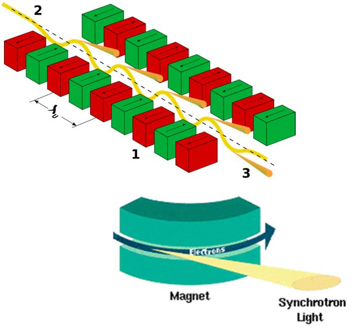
17 Angula distibution dp t n t n t t t β β 1 e 4πε 4π 1 β dω n t t n ( n β β β( osθ β osφθ ˆ + βsinφ( 1 βosθ ˆ φ dp t 1 e β sin θos φ 1 dω 4πε 4π 1 βosθ γ 1 βosθ 5 4 Fo γ << θ << 1and γ >> 1, it an be shown that the angula spead of the adiation powe is ~ γ 1. (Homewok poblem β βεˆ β sinθ osφ + θosθosφ φsinφ 1 ( n ˆ ˆ β βεˆ β osθ θsinθ ( n ˆ n ˆ

18 Angula distibution β β β β. β. β.8 β * These plots show how the length of a veto,, depends on its dietion ( θ, φ. Sine the length has the same dietional dependane as the powe, we an see the angula distibution of powe by looking at the length of the veto along all dietions. (Spheial D plot in Mathematia β 1 sin θos φ 1 ( 1 β osθ γ ( 1 βosθ β

19 Spetum In ode to get the fequeny ontents of the adiation, o the spetum, we need to do Fouie tansfomations. a x t R t E x t (, ε (, ( dp t dω ad 1 a ( x, t a ( x, t dωdω' a( x, ω a ( x, ω' e e π 1 iωt a( x, t a ( x, ω e dω π * iω ' t iωt Now we alulate the total enegy pe solid angle eeived at the obsevation point ( dp t d I ( ω dw dt a ( x, ω dω dω dω dω dωdω Spetum intensity: enegy eeived pe solid angle pe fequeny inteval d I ( ω dωdω a x, ( ω

20 Spetum II To poeed, we need to alulate the Fouie omponents of the 1 eleti field: (, (, i t a ω x ω a x t e dt e β n( t e ( n( t β( t β( t i ( t R( t / a ω + ( x, ω e dt 4π πε 1 n( t β ( t iωe ixω/ iω( t n ( t / e n( t ( n( t β ( t e dt 4π πε (( n β β ( β d n ( n β n dt ( 1 n β 1 n π (, a x t Fa field appoximation, ( E τ << x ( β 4 R t 1 n t t β n ( τ R ( τ ( x ( τ ( x ( τ x 1 R τ x n t x ad πε n n t t t ( ω di 1 ω e ( iω( t n ( t / a x, ω n n β e dt dωdω 4πε 4π

21 Spetum III ω t << 1 Polaization of eleti field is deomposed into a ( x, ω a ( x, ω ˆ ε a// ( x, ω ˆ + ε// E x ω E x ω ε E x ω ˆ ε (, (, ˆ + (, // // ˆ ε : inside the obit plane of patile // ˆ : nealy pependiula to the obit plane ε 1 n( t sin ˆ ˆ ˆ ˆ n t β t β θε βω tε// βθε βω tε θ // ( ω t ( ω t β β β β ( t sin ( ˆ1 os( ˆ ˆ ˆ ˆ ω t ε ω t ε ε ωt ε1 ε ω + + ω ω 6 ω ω 1 ω t n( t ( t / ω t + θ + ( ω t ω γ 1 γ <<

22 Spetum IV ( ω 1 ω e ω 1 ( ωt ( βθεˆ ˆ βω tε// exp i ωt + θ + dt ω Ω 4πε 4π ω γ d I d d 1 ω e θ βθεˆ I η θ βε // // η 4πε 4π ω γ + γ ˆ I 1 ω 1 ω ( 1 ω γ ω η + θ + γ θ Citial fequeny ρ ω γ γ ω I i η x x dx K ( I η xexp i x+ x dx K ( η // ( η exp ( + ( η 1 η i x ωεˆ Contibution fom E (, // // d I ω 1 e γ ω θ γ ( 1+ γ θ K1 ( η + K ( η dωdω 4πε 4π ω ( 1+ θγ x ω ε Contibution fom E (, ˆ ω ω γθ Fo θ, using the asymptoti appoximation of Bessel funtion, 1 1 e γ 4 ω Γ ; ω<< ω 4πε 4π ω ( ω 1 e γ ω K ( η ω Ω 4πε 4π ω ω 1 e γ ω ω e ; ω >> 4πε 4π ω d I d d ω

23 Enegy spetum V The total enegy spetum is obtained by integating ove the solid angle: π π γ ( ω π d I( ω dw d I π osθdθ d( γθ dω dωdω γ dωdω π π γ e γω y ω ω ( 1 1 ( 1 ( y K + y + K + y dy 4πε π ω ( 1+ y ω ω A moe onise and popula expession fo the enegy spetum: dw 1 e γ ω K dω 4πε ω ωω 5 / x dx

24 Homewok Conside an eleton stoage ing at an enegy of 1 GeV, a iulating uent of ma and a bending adius of ρ.m. Calulate the enegy loss pe tun, the itial photon enegy, and the total synhoton adiation powe. Make a shot agument about why the tajetoy of a haged patile an not inteset with light one moe than one (see slide #8.

25 Homewok As shown in slide #15, the angula distibution of adiation powe is dp t 1 e β sin θos φ 1 dω 4πε 4π 1 βosθ γ 1 βosθ 4 Show that fo γ << θ << 1 and γ >> 1, the angula spead of the adiation powe is in the ode of γ 1.