The Friction Stir Welding Process

HTML
DOWNLOAD

Μέγεθος: px

Εμφάνιση ξεκινά από τη σελίδα:

Download "The Friction Stir Welding Process"

Ζέφυρ Βιτάλης
6 χρόνια πριν
Προβολές:

1 1 / 27 The Fiction Sti Welding Pocess Goup membes: Kik Fase, Sean Bohun, Xiulei Cao, Huaxiong Huang, Kate Powes, Aina Rakotondandisa, Mohammad Samani, Zilong Song 8th Monteal Industial Poblem Solving Wokshop 11 August 2017

2 The FSW pocess 2 / 27

3 The Fou Phases of Ceating a Weld 3 / 27

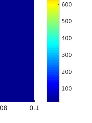
4 Mechanisms of Welding Steady State: Heat Shea flow Applied pessue Plastic/elastic Paametes: Aluminium k 237 E 70 ν 0.35 ρ 2700 cp 897 Steel J/s.m.K GPa kg/m3 J/kg.K 4 / 27

5 5 / 27 Heat What Role Does Heat Play?

6 6 / 27 The heat model Newtonian Cooling ρc T t = 1 dt p ρ p c p dt = q p [ k T ] + q s (p, s] + h ps (T p T s ) + h p (T p T p ) p V p V p ρ s c s dt s dt = h ps V s (T p T s ) + h s V s (T s T (p, s])

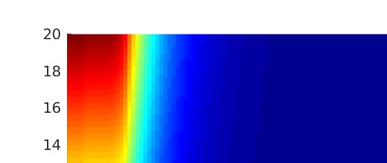
7 The Heat Equation 7 / 27

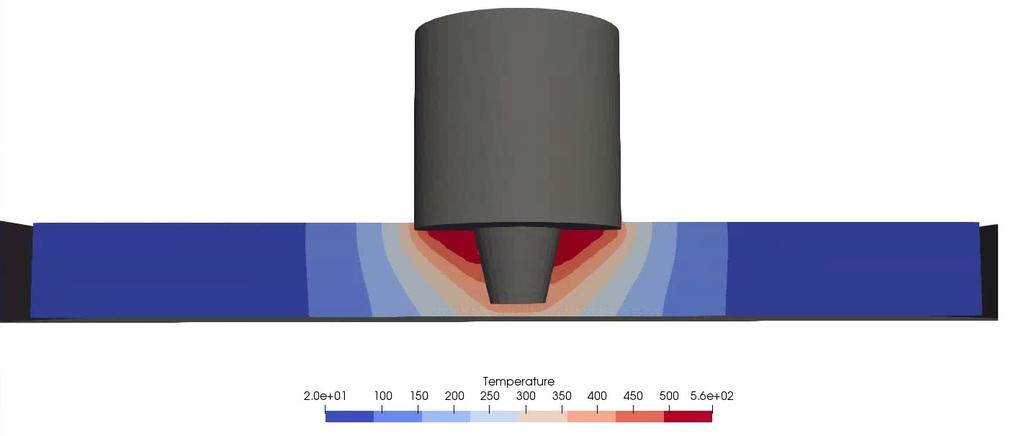
8 8 / 27 Lessons Leaned 1 The shoulde is mostly esponsible fo heating, not the pin. 2 The heat loss though the tool is significant. 3 The heat does not tavel too fa in the diection, due to the lage heat capacity of the mateial. 4 The effect of yielding mateial should be taken into consideation to avoid the constant ise in tempeatue. The mateial should yield in less than 10 s.

9 9 / 27 Plastic/Elastic Plastic / Elastic

10 Elastic/Plastic 10 / 27

11 11 / 27 Elastic/Plastic Equations Elastic equations σ = 0 (1) σ = Cε (2) ε = 1 2 ( u + ut ) (3) Heat Equation ρc DT = (k T ) + σ : ε (4) Dt Plastic equations σ = ρ D v Dt v = 0 (5) ε = Λ σ y (σ 1 3 T(σ)I) = Λ σ y σ dev (6) σy(t 2 ) = 3 2 σdev ij σij dev (7)

12 Plastic I ( p b ) Foce balance: v = v (), v θ (), 0 ( ) v ρ t + v v v2 θ ( vθ ρ t + v v θ + v ) v θ v + v Constitutive elation: σ = p + σ y v Λ, σ θ = σ ( y vθ 2Λ v θ = σ + 1 (σ σ θθ ), (8) = σ θ + 2 σ θ, (9) = 0. (10) σ θθ = p + σ y v Λ, (11) ), p = 1 3 (σ + σ θθ + σ zz ), (12) (σ p) 2 + (σ θθ p) 2 + (σ zz p) 2 + 2σ 2 θ = 2σ2 y 3. (13) 12 / 27

13 13 / 27 Elastic I ( b L) Foce balance: u = u (), u θ (), 0 Constitutive elation: 0 = σ + 1 (σ σ θθ ), (14) 0 = σ θ + 2 σ θ. (15) σ = (λ + 2µ)ε + λε θθ, σ θ = 2µε θ, (16) σ θθ = (λ + 2µ)ε θθ + λε, σ zz = λ(ε θθ + ε ), (17) ε = u, ε θ = 1 ( uθ 2 u ) θ, (18) ε θθ = u. (19)

14 14 / 27 Bounday conditions = p : v θ = γω p, (20) σ θ = fσ. (21) = L: σ = 0, (22) σ θ = 0. (23) = b : v θ = 0, (24) p = p b, (25) [σ ] = 0, (26) [σ θ ] = 0. (27)

15 15 / 27 Solution fo the elastic defomation in steady state σ = σ b b 2, 2 u = σ b 1+ν E σ θθ = σ b b 2 2, 2 b, u θ = σ b θ 1+ν E σ θ = σθ b b 2, (28) 2 2 b (29)

16 16 / 27 Solution fo the plastic defomation in steady state Incompessibility gives v = c 1, and fom the flow elations ( ) 3σyc Λ = ( ) 4 σy 2 3σθ 2. Shea foce balance gives σ θ = ρc 1v θ and the emaining flow elation gives ( v θ 1 = + 2Λρc 1 σ y with the foce balance giving σ = 2σ yc 1 Λ 3 ρc2 1 3 ρv2 θ, + c 2 2, ) v θ + 2Λc 2 σ y 2, v θ = { γω p at p 0 at b, { σ θ = fσ at p p = p b at b. (30) (31)

17 Solution fo the plastic defomation in steady state 17 / 27

18 Solution fo the plastic defomation in steady state 18 / 27

19 Solution fo the elastic/plastic defomation 19 / 27

20 20 / 27 Lessons leaned If v = 0 (stationay at pin) solution does not exist If v > 0 (unphysical) then v is huge Inconsistency of plastic flow with incompessible fluid Pehaps a shea stess condition at p is unwise

21 Plastic II Equations: 0 = dσ d + 1 (σ σ θθ ), (32) 0 = dσ θ d + 2 σ θ, (33) 1 4 (σ σ θθ ) 2 + σθ 2 = σ2 y(t ) (34) Bounday conditions: Solutions: σ = P 0, σ θ = fσ, = p. (35) σ θ () = fp 0 p/ 2 2, (36) σ () = 2 p s σy 2 σθ 2 (s)ds + P 0, (37) σ θθ = σ ± 2 σy 2 σθ 2 (). (38) Use yield citeion and two matching conditions [σ ] = [σ θ ] = 0 to detemine b and σ, b σθ b. Decouples flow and stess. Tempeatue could be useful: σ y = σ y () 21 / 27

22 22 / 27 Stokes Flow + Heat Equation Numeical simulation with finite element method using Stokes model. (2µ ε) p = 0, (39) v = 0, (40) ρc DT Dt (k T ) Q = 0 (41) Q = α dissipation σ dev : ε with σ dev = 2µ ε (42) ε = 1 2 ( T (v) + (v)) (43) Noton-Hoff law: µ = K(T )(2 ε : ε + 3γ 2 m(t ) 1 ) 2. We assume K and m constant: K = 10 6 and m = 0.2, γ = 10 3.

23 T Numeical simulation with finite element method Tempeatue v θ v θ v 0.5 v Stess components seem unstable. Bounday laye? Tempeatue is uncoupled. Still need K = K(T ), m = m(t ). 23 / 27

24 v θ = 0, v = 0, at = L. 24 / 27 Numeical simulation fo plastic defomation FV We deive the following system with the unkowns (v, v θ, Λ, p) ρ v t + (ρv σ y Λ ) v (σ y Λ ρ v θ t + (ρv σ y Λ ) v θ + ( σ y 2Λ v θ σ y 2Λ Λ = 3 ( 2 2 ( v v ) σ y + Λ 2 v = ρ v2 θ + p, ) 2 1( v θ + 2 v θ ) ) 2, v θ ) (ρv + + σ y ) vθ Λ 3 = 0, and ( p) ( = ( σ y Λ v ) 2σ y + Λ v v ) + ρv ρv2 θ closed by the bounday conditions v θ = γ p ω, σ = 10 5, at = p,

25 25 / 27 Numeical simulation fo plastic defomation FV To be done late: pessue equation is unstable.

26 26 / 27 Poposed consistent mechanism Plasticize egion with pessue σ zz Heating is seconday u z o u θ z is impotant (may esolve incompessibility poblem) Tanslation of pin within plastic egion geneates flow Shea flow blending the mateial

27 Thank you! 27 / 27

Σχετικά έγγραφα

21. Stresses Around a Hole (I) 21. Stresses Around a Hole (I) I Main Topics

21. Stresses Around a Hole (I) 21. Stresses Around a Hole (I) I Main Topics I Main Topics A Intoducon to stess fields and stess concentaons B An axisymmetic poblem B Stesses in a pola (cylindical) efeence fame C quaons of equilibium D Soluon of bounday value poblem fo a pessuized