Modern Regression HW #8 Solutions

Μέγεθος: px

Εμφάνιση ξεκινά από τη σελίδα:

Download "Modern Regression HW #8 Solutions"

Ἰωνᾶς Μαρκόπουλος
5 χρόνια πριν
Προβολές:

1 36-40 Modern Regression HW #8 Solutions Problem [25 points] (a) DUE: /0/207 at 3PM This is still a linear regression model the simplest possible one. That being the case, the solution we derived before β = ( T ) T Y still holds. The design matrix is so =., β = ( T ) }{{}} T {{ Y } /n = Y i = Y. (b) So H = ( T ) T = (. (n) ) n n n. =... n..... n n n h ii = n for all i =,..., n.

2 (c) Ŷ = HY n n i= Y i =. = n n i= Y i Y. Y (d) t i = Y i Ŷi( i) s i Y i n j n j i Y i = Var(Y i ( Ŷi( i)) n ) Y i n Y j Y i j= = Var(Y i ) + Var(Ŷi( i)) = Y ( ) i ny n Yi σ 2 + σ2 n = Y ( ) i ny n Yi = nσ 2 n n n (Y i Y ) nσ 2 n (e) lim t i = Y i = lim Y i = n n (Y i Y ) nσ 2 n n n (lim Y i Y i Y ) nσ 2 n 2

3 Problem 2 [20 points] H = HH h h 2 h n h h 2 h n h h 2 h n h 2 h 22 h 2n..... = h 2 h 22 h 2n h 2 h 22 h 2n h n h nn h n h nn h n h nn So for each diagonal element of H we have, h ii = h 2 ii + h 2 ij. j i We have expressed h ii as a sum of squares, so h ii 0. Furthermore, so h ii h 2 ii, h ii. 3

4 Problem 3 [20 points] Comments omitted. One of the points in data set four produces NaN s because it has leverage. See equation (2) of Lecture Notes 20. attach(anscombe) names(anscombe) ## [] "x" "x2" "x3" "x4" "y" "y2" "y3" "y4" Y Residuals Figure : Data Set 4

5 Y Residuals Figure 2: Data Set 2 5

6 Y Residuals Figure 3: Data Set 3 6

7 Y Residuals Figure 4: Data Set 4 7

8 Problem 4 [25 points] Discussions omitted (i) y age tri chol (ii) model <- lm(y ~ age + tri + chol, data = data) 8

9 (iii) Age Age Triglycerides Triglycerides Cholesterol Cholesterol 9

10 (iv) model <- lm(y ~ age + tri + chol + I(age^2) + I(tri^2) + I(chol^2), data = data) Age Age Triglycerides Triglycerides Cholesterol Cholesterol 0

11 which(rstudent(model) > 30) ## 25 ## 25 (v) data2 <- data[-25,] model <- lm(y ~ age + tri + chol + I(age^2) + I(tri^2) + I(chol^2), data = data2) Age Age Triglycerides Triglycerides

12 Cholesterol Cholesterol library(knitr) kable(summary(model)$coefficients) Estimate Std. Error t value Pr(> t ) (Intercept) age tri chol I(ageˆ2) I(triˆ2) I(cholˆ2) kable(confint(model, parm = 2:6, level = / 6)) 0.47 % % age tri chol I(ageˆ2) I(triˆ2)

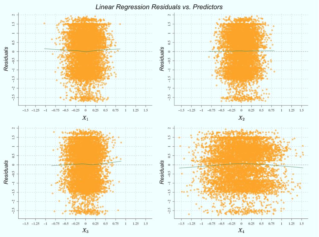
13 Problem 5 [0 points] d = read.table(" y = d[,] x = d[,2] x2 = d[,3] x3 = d[,4] x4 = d[,5] (a) y x x x Figure 5: Secret Data (b) model5 <- lm(y ~ x + x2 + x3 + x4) Summarize the fitted model x

14 4

15 5

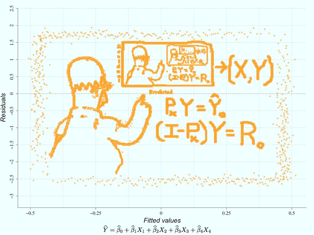
16 Figure 6: The above residual plot is a spoof of this scene from The Simpsons Appendix quartz(height = 2, width = 6) par(mar = c(4,4.5,2,2) + 0.) par(oma = c(.5,,2,) + 0.) par(mfrow=c(2,2)) par(bg = "azure") out <- lm(y ~ x+x2+x3+x4) plot(x, residuals(out), col = NA, pch = 9, axes = FALSE, ylab = "Residuals", font.lab = 3, xlab = "", xlim = range(x4), cex.lab=2) axis(side =, at = seq(-2.5,2.5,0.25), labels = as.character(seq(-2.5,2.5,0.25)), font = 5, cex.axis =.25) axis(side = 2, at = seq(-3,2.5,0.5), labels = as.character(seq(-3,2.5,0.5)), font = 5, cex.axis =.25) abline(h = seq(-3,2.5,0.5), col = "gray75", lty = 2) abline(v = seq(-2.5,2.5,0.25), col = "gray80", lty = 2) 6

17 abline(0,0, lty = 2, col = "gray45") points(x, residuals(out), col = addtrans("orange",20), pch = 9) points(x, residuals(out), col = "orange") panel.smooth(x, residuals(out), col = "orange",cex =, lwd =.2, col.smooth = "seagreen", span = 2/3, iter = 3) plot(x2, residuals(out), col = NA, pch = 9, axes = FALSE, ylab = "Residuals", font.lab = 3, xlab = "", xlim = range(x4), cex.lab=2) axis(side =, at = seq(-2.5,2.5,0.25), labels = as.character(seq(-2.5,2.5,0.25)), font = 5, cex.axis =.25) axis(side = 2, at = seq(-3,2.5,0.5), labels = as.character(seq(-3,2.5,0.5)), font = 5, cex.axis =.25) abline(h = seq(-3,2.5,0.5), col = "gray75", lty = 2) abline(v = seq(-2.5,2.5,0.25), col = "gray80", lty = 2) abline(0,0, lty = 2, col = "gray45") points(x2, residuals(out), col = addtrans("orange",20), pch = 9) points(x2, residuals(out), col = "orange") panel.smooth(x2, residuals(out), col = "orange",cex =, lwd =.2, col.smooth = "seagreen", span = 2/3, iter = 3) plot(x3, residuals(out), col = NA, pch = 9, axes = FALSE, ylab = "Residuals", font.lab = 3, xlab = "", xlim = range(x4), cex.lab=2) axis(side =, at = seq(-2.5,2.5,0.25), labels = as.character(seq(-2.5,2.5,0.25)), font = 5, cex.axis =.25) axis(side = 2, at = seq(-3,2.5,0.5), labels = as.character(seq(-3,2.5,0.5)), font = 5, cex.axis =.25) abline(h = seq(-3,2.5,0.5), col = "gray75", lty = 2) abline(v = seq(-2.5,2.5,0.25), col = "gray80", lty = 2) abline(0,0, lty = 2, col = "gray45") points(x3, residuals(out), col = addtrans("orange",20), pch = 9) points(x3, residuals(out), col = "orange") panel.smooth(x3, residuals(out), col = "orange",cex =, lwd =.2, col.smooth = "seagreen", span = 2/3, iter = 3) plot(x4, residuals(out), col = NA, pch = 9, axes = FALSE, ylab = "Residuals", font.lab = 3, xlab = "", xlim = range(x4), cex.lab=2) axis(side =, at = seq(-2.5,2.5,0.25), labels = as.character(seq(-2.5,2.5,0.25)), font = 5, cex.axis =.25) axis(side = 2, at = seq(-3,2.5,0.5), labels = as.character(seq(-3,2.5,0.5)), font = 5, cex.axis =.25) abline(h = seq(-3,2.5,0.5), col = "gray75", lty = 2) abline(v = seq(-2.5,2.5,0.25), col = "gray80", lty = 2) abline(0,0, lty = 2, col = "gray45") points(x4, residuals(out), col = addtrans("orange",20), pch = 9) points(x4, residuals(out), col = "orange") panel.smooth(x4, residuals(out), col = "orange",cex =, lwd =.2, col.smooth = "seagreen", span = 2/3, iter = 3) mtext("linear Regression Residuals vs. Predictors", side = 3, line = -.2, outer = TRUE, font = 3, cex = 2) quartz.save(file = "residuals.png", type = "png") graphics.off() 7

18 quartz(height = 2, width = 6) par(mar = c(7,4.5,2,2) + 0.) par(bg = "azure") par(mfrow=c(,)) plot(out, which =, col = NA, pch = 9, axes = FALSE,add.smooth = FALSE, caption = "", font.lab = 3, sub.caption = "", cex.lab = 2, labels.id = NA) axis(side =, at = seq(-3,2.5,0.25), labels = as.character(seq(-3,2.5,0.25)), font = 5, cex.axis =.5) axis(side = 2, at = seq(-3.5,2.5,0.5), labels = as.character(seq(-3.5,2.5,0.5)), font = 5, cex.axis =.5) abline(h = seq(-3,2.5,0.5), col = "gray75", lty = 2) abline(v = seq(-2.5,2.5,0.25), col = "gray80", lty = 2) abline(0,0, lty = 2, col = "gray45") points(fitted(out), residuals(out), col = addtrans("orange",20), pch = 9, cex = 0.8) points(fitted(out), residuals(out), col = "orange", cex = 0.8) quartz.save(file = "homer.png", type = "png") 8

Σχετικά έγγραφα

DirichletReg: Dirichlet Regression for Compositional Data in R

DirichletReg: Dirichlet Regression for Compositional Data in R Marco J. Maier Wirtschaftsuniversität Wien Abstract Full R Code for Maier, M. J. (2014). DirichletReg: Dirichlet Regression for Compositional