- PDF Free Download

Μέγεθος: px

Εμφάνιση ξεκινά από τη σελίδα:

Download ""

Ἑκάβη Γούναρης
6 χρόνια πριν
Προβολές:

6 X = [ ] X X double[] X = { 1, 2, 4, 6, 12, 15, 25, 45, 68, 67, 65, 98 }; double X.Length double

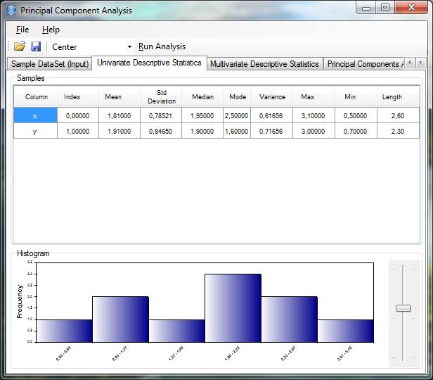
7 double[] x1 = { 0, 8, 12, 20 }; double[] x2 = { 8, 9, 11, 12 }; double mean1 = x1.mean(); double mean2 = x2.mean(); double stddev1 = x1.standarddeviation(); double stddev2 = x2.standarddeviation(); double stddev1 = x1.standarddeviation(mean1); double stddev2 = x2.standarddeviation(mean2);

8 // Create some sets of numbers double[] x1 = { 0, 8, 12, 20 }; double[] x2 = { 8, 9, 11, 12 }; // Compute the means double mean1 = x1.mean(); double mean2 = x2.mean(); // Compute the standard deviations double stddev1 = x1.standarddeviation(mean1); double stddev2 = x2.standarddeviation(mean2); Data: x1: x2: Means: x1: 10 x2: 10 Standard Deviations: x1: x2: // Show results on screen Console.WriteLine("Data:"); Console.WriteLine(" x1: " + x1.tostring("g")); Console.WriteLine(" x2: " + x2.tostring("g")); Console.WriteLine("Means:"); Console.WriteLine(" x1: " + mean1); Console.WriteLine(" x2: " + mean2); Console.WriteLine("Standard Deviations:"); Console.WriteLine(" x1: " + stddev1); Console.WriteLine(" x2: " + stddev2);

9 StandardDeviation() Variance() double cov = x1.covariance(x2);

10 double[,] data = { // Hours (H) Mark (M) { 9, 39 }, { 15, 56 }, { 25, 93 }, { 14, 61 }, { 10, 50 }, { 18, 75 }, { 0, 32 }, { 16, 85 }, { 5, 42 }, { 19, 70 }, { 16, 66 }, { 20, 80 } }; double[,] covariancematrix = data.covariance(); ScatterplotBox.Show(data);

11 double[,] data = { // Hours (H) Mark (M) { 9, 39 }, { 15, 56 }, { 25, 93 }, { 14, 61 }, { 10, 50 }, { 18, 75 }, { 0, 32 }, { 16, 85 }, { 5, 42 }, { 19, 70 }, { 16, 66 }, { 20, 80 } }; // Compute total and average double[] totals = data.sum(); double[] averages = data.mean(); Data: Hours(H) Mark(M) Sum: Avg: Covariance matrix: // Compute covariance matrix double[,] C = data.covariance(); // Show results on screen Console.WriteLine("Data: "); Console.WriteLine(" Hours(H) Mark(M)"); Console.WriteLine(data.ToString(" 00")); Console.WriteLine("Sum: " + totals.tostring("000.00")); Console.WriteLine("Avg: " + averages.tostring(" 00.00")); Console.WriteLine("Covariance matrix:"); Console.WriteLine(C.ToString(" ")); Console.ReadKey(); ScatterplotBox.Show(data);

13 // Consider the following matrix double[,] A = { { 2, 3 }, { 2, 1 } }; // Now consider the vector double[] u = { 1, 3 }; // Multiplying both, we get x = [ 11 5 ]' double[] x = A.Multiply(u); // We can not express 'x' as a multiple // of 'u', so 'u' is not an eigenvector. // However, consider now the vector double[] v = { 3, 2 }; // Multiplying both, we get y = [ 12 8 ]' double[] y = A.Multiply(v); Matrix A: Vector u: 1 3 Vector v: 3 2 x = A*u 11 5 y = A*v 12 8 // It can be seen that 'y' can be expressed as // a multiple of 'v'. Since y = 4*v, 'v' is an // eigenvector with the associated eigenvalue 4. // Show on screen Console.WriteLine("Matrix A:"); Console.WriteLine(A.ToString(" 0")); Console.WriteLine("Vector u:"); Console.WriteLine(u.Transpose().ToString(" 0")); Console.WriteLine("Vector v:"); Console.WriteLine(v.Transpose().ToString(" 0")); Console.WriteLine("x = A*u"); Console.WriteLine(x.Transpose().ToString(" 0")); Console.WriteLine("y = A*v"); Console.WriteLine(y.Transpose().ToString(" 0"));

14 A n n A v n Av = λv. λ v v v A λ v V V A Λ Λ A = V Λ V A V A = V Λ V M = ( 2 0 2) 4 2 3

15 M ( 0 ) = ( 2 0 2) ( 0 ) = ( 0 ) M v = ( 1,0, 1) (1, 0, 1) v v (λ, v ) λ = 1 v = ( 1,0, 1) 1 Λ V

16 // Consider the following matrix double[,] M = { { 3, 2, 4 }, { 2, 0, 2 }, { 4, 2, 3 } }; // Create an Eigenvalue decomposition var evd = new EigenvalueDecomposition(M); // Store the eigenvalues and eigenvectors double[] λ = evd.realeigenvalues; double[,] V = evd.eigenvectors; // Reconstruct M = V*λ*V' double[,] R = V.MultiplyByDiagonal(λ).MultiplyByTranspose(V); Matrix: Eigenvalues: Eigenvectors: Reconstruction: // Show on screen Console.WriteLine("Matrix: "); Console.WriteLine(M.ToString(" 0")); Console.WriteLine("Eigenvalues: "); Console.WriteLine(λ.ToString(" ; ;")); Console.WriteLine("Eigenvectors:"); Console.WriteLine(V.ToString(" ; ;")); Console.WriteLine("Reconstruction:"); Console.WriteLine(R.ToString(" 0"));

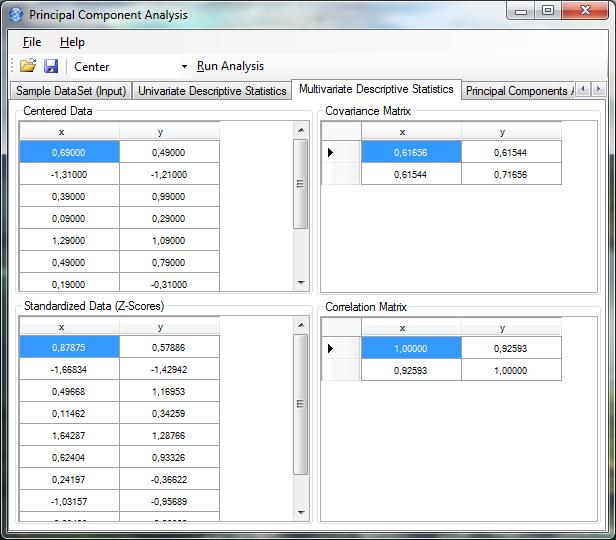
18 double[,] data = { { 2.5, 2.4 }, { 0.5, 0.7 }, { 2.2, 2.9 }, { 1.9, 2.2 }, { 3.1, 3.0 }, { 2.3, 2.7 }, { 2.0, 1.6 }, { 1.0, 1.1 }, { 1.5, 1.6 }, { 1.1, 0.9 } }; double[] mean = data.mean(); double[,] dataadjust = data.subtract(mean); Data = x y dataadjust = x y

19 double[,] cov = dataadjust.covariance(); cov cov = ( ) var evd = new EigenvalueDecomposition(cov); double[] eigenvalues = evd.realeigenvalues; double[,] eigenvectors = evd.eigenvectors; // Sort eigenvalues and vectors in descending order eigenvectors = Matrix.Sort(eigenvalues, eigenvectors, new GeneralComparer(ComparerDirection.Descending, true)); eigenvalues = ( ) eigenvectors = ( )

20 double[,] featurevector = eigenvectors; double[,] featurevector = eigenvectors.getcolumn(0).transpose(); double[,] finaldata = dataadjust.multiply(eigenvectors); 1 st PC 2 nd PC st PC

21 // Step 1. Get some data double[,] data = { { 2.5, 2.4 }, { 0.5, 0.7 }, { 2.2, 2.9 }, { 1.9, 2.2 }, { 3.1, 3.0 }, { 2.3, 2.7 }, { 2.0, 1.6 }, { 1.0, 1.1 }, { 1.5, 1.6 }, { 1.1, 0.9 } }; // Step 2. Subtract the mean double[] mean = data.mean(); double[,] dataadjust = data.subtract(mean); // Step 3. Calculate the covariance matrix double[,] cov = dataadjust.covariance(); // Step 4. Calculate the eigenvectors and // eigenvalues of the covariance matrix var evd = new EigenvalueDecomposition(cov); double[] eigenvalues = evd.realeigenvalues; double[,] eigenvectors = evd.eigenvectors; // Step 5. Choosing components and // forming a feature vector // Sort eigenvalues and vectors in descending order eigenvectors = Matrix.Sort(eigenvalues, eigenvectors, new GeneralComparer(ComparerDirection.Descending, true)); // Select all eigenvectors double[,] featurevector = eigenvectors; // Step 6. Deriving the new data set double[,] finaldata = dataadjust.multiply(eigenvectors); Data x y Data Adjust x y Covariance Matrix: Eigenvalues: Eigenvectors: Transformed Data x y

22 // Show on screen Console.WriteLine("Data"); Console.WriteLine(" x y"); Console.WriteLine(" "); Console.WriteLine(data.ToString(" 0.0 ")); Console.ReadKey(); Console.WriteLine("Data Adjust"); Console.WriteLine(" x y"); Console.WriteLine(" "); Console.WriteLine(dataAdjust.ToString(" 0.00; -0.00;")); Console.ReadKey(); ScatterplotBox.Show("Original PCA data", data); Console.ReadKey(); Console.WriteLine("Covariance Matrix: "); Console.WriteLine(cov.ToString(" ; ;")); Console.WriteLine("Eigenvalues: "); Console.WriteLine(eigenvalues.ToString(" ; ;")); Console.WriteLine("Eigenvectors:"); Console.WriteLine(eigenvectors.ToString(" ; ;")); Console.ReadKey(); Console.WriteLine("Transformed Data"); Console.WriteLine(" x y"); Console.WriteLine(" "); Console.WriteLine(finalData.ToString(" ; ;")); ScatterplotBox.Show("Transformed PCA data", finaldata);

23 A m n A U Σ V A = U Σ V U V Σ A C = 1 n 1 A A. C A A A A A A A = V Λ V Λ = Σ Σ A A = V Λ V = V (Σ Σ) V A A

24 U I = U U A A = V Λ V = V Σ Σ V = V Σ I Σ V = V Σ U U Σ V A = V Σ U A = U Σ V A A (V Σ U )( U Σ V ) = A A ( U Σ V )(V Σ U ) = AA V A A U AA Σ A A AA double[,] data = { { 2.5, 2.4 }, { 0.5, 0.7 }, { 2.2, 2.9 }, { 1.9, 2.2 }, { 3.1, 3.0 }, { 2.3, 2.7 }, { 2.0, 1.6 }, { 1.0, 1.1 }, { 1.5, 1.6 }, { 1.1, 0.9 } };

25 double[] mean = data.mean(); double[,] dataadjust = data.subtract(mean); Data = x y dataadjust = x y var svd = new SingularValueDecomposition(dataAdjust); double[] singularvalues = svd.diagonal; double[,] eigenvectors = svd.rightsingularvectors; singularvalues = ( ) eigenvectors = ( )

26 double[] eigenvalues = singularvalues.elementwisepower(2); A A n 1 A A eigenvalues = eigenvalues.divide(data.getlength(0) - 1); eigenvalues = ( )

27 // Step 1. Get some data double[,] data = { { 2.5, 2.4 }, { 0.5, 0.7 }, { 2.2, 2.9 }, { 1.9, 2.2 }, { 3.1, 3.0 }, { 2.3, 2.7 }, { 2.0, 1.6 }, { 1.0, 1.1 }, { 1.5, 1.6 }, { 1.1, 0.9 } }; // Step 2. Subtract the mean double[] mean = data.mean(); double[,] dataadjust = data.subtract(mean); // Step 3. Calculate the singular values and // singular vectors of the data matrix var svd = new SingularValueDecomposition(dataAdjust); double[] singularvalues = svd.diagonal; double[,] eigenvectors = svd.rightsingularvectors; // Step 4. Calculate the eigenvalues as // the square of the singular values double[] eigenvalues = singularvalues.elementwisepower(2); // Step 5. Choosing components and // forming a feature vector // Select all eigenvectors double[,] featurevector = eigenvectors; // Step 6. Deriving the new data set double[,] finaldata = dataadjust.multiply(eigenvectors); Data x y Data Adjust x y Singular values: Eigenvalues: Eigenvalues (normalized): Eigenvectors: Transformed Data x y

28 // Show on screen. Console.WriteLine("Data"); Console.WriteLine(" x y"); Console.WriteLine(" "); Console.WriteLine(data.ToString(" 0.0 ")); Console.ReadKey(); Console.WriteLine("Data Adjust"); Console.WriteLine(" x y"); Console.WriteLine(" "); Console.WriteLine(dataAdjust.ToString(" 0.00; -0.00;")); Console.ReadKey(); ScatterplotBox.Show("Original PCA data", data); Console.WriteLine("Singular values: "); Console.WriteLine(singularValues.ToString(" ; ;")); Console.WriteLine("Eigenvalues: "); Console.WriteLine(eigenvalues.ToString(" ; ;")); // Normalize eigenvalues to replicate the covariance eigenvalues = eigenvalues.divide(data.getlength(0) - 1); Console.WriteLine("Eigenvalues (normalized): "); Console.WriteLine(eigenvalues.ToString(" ; ;")); Console.WriteLine("Eigenvectors:"); Console.WriteLine(eigenvectors.ToString(" ; ;")); Console.ReadKey(); Console.WriteLine("Transformed Data"); Console.WriteLine(" x y"); Console.WriteLine(" "); Console.WriteLine(finalData.ToString(" ; ;"));

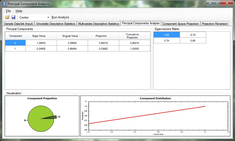
29 var pca = new PrincipalComponentAnalysis(data); pca.overwrite = true; pca.method = AnalysisMethod.Standardize; pca.compute();

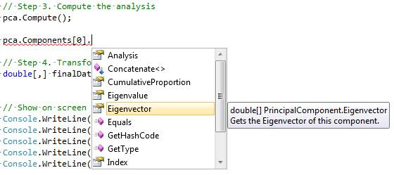
30 datagridview1.datasource = pca.components;

32 // Step 1. Get some data double[,] data = { { 2.5, 2.4 }, { 0.5, 0.7 }, { 2.2, 2.9 }, { 1.9, 2.2 }, { 3.1, 3.0 }, { 2.3, 2.7 }, { 2.0, 1.6 }, { 1.0, 1.1 }, { 1.5, 1.6 }, { 1.1, 0.9 } }; // Step 2. Create the Principal Component Analysis var pca = new PrincipalComponentAnalysis(data); // Step 3. Compute the analysis pca.compute(); // Step 4. Transform your data double[,] finaldata = pca.transform(data); // Show on screen Console.WriteLine("Data"); Console.WriteLine(" x y"); Console.WriteLine(" "); Console.WriteLine(data.ToString(" 0.0 ")); Console.ReadKey(); ScatterplotBox.Show("Original PCA data", data); Console.WriteLine("Eigenvalues: "); Console.WriteLine(pca.Eigenvalues.ToString(" ; ;")); Console.WriteLine("Eigenvectors:"); Console.WriteLine(pca.ComponentMatrix.ToString(" ; ;")); Console.ReadKey(); Console.WriteLine("Transformed Data"); Console.WriteLine(" x y"); Console.WriteLine(" "); Console.WriteLine(finalData.ToString(" ; ;")); Data x y Eigenvalues: Eigenvectors: Transformed Data x y

Σχετικά έγγραφα

( ) 2 and compare to M.

( ) 2 and compare to M. Problems and Solutions for Section 4.2 4.9 through 4.33) 4.9 Calculate the square root of the matrix 3!0 M!0 8 Hint: Let M / 2 a!b ; calculate M / 2!b c ) 2 and compare to M. Solution: Given: 3!0 M!0 8