Christian J. Bordé SYRTE & LPL.

HTML
DOWNLOAD

Μέγεθος: px

Εμφάνιση ξεκινά από τη σελίδα:

Download "Christian J. Bordé SYRTE & LPL."

Μνάσων Δεσποτόπουλος
6 χρόνια πριν
Προβολές:

1 Relativisti atom optis and interferometry : a trip in the fifth dimension Christian J. Bordé SYRTE & LPL

2 1 t Δ

3 ENERGY E( p) M + p 4 hν db E(p) Ω atom slopev M p p M ϕ+ ϕ rest mass hν M photon slope h / λ h / λdb MOMENTUM p K

4 KLEIN-GORDON EQUATION (Curved spae-time) ϕ M + 1/ 1/ ( ) ( ) ϕ g ν ϕ g g g ν ϕ ν ν g η + h with h << 1 ν ν ν ν 1 Δ h ν t ν

5 Elementary interval ν ds ν dx, (time),1,,3 (spae) Metri tensor 1 h 1 g ν + 1 sym 1 Analogy with: A ( V, A) Post-Newtonian parameters (PPN): g h i dx - gravitation field: h g. r / r. γ. r / - rotation field: h Ω r / U - gravitational wave: h h ν h h 1 11 h h h γ β U h h h h U δ i +..

6 LASER POINTER AND D OPTICS ϕ x ik x ϕ ϕ 1 ϕ ϕ ϕ + k ϕ x t y z ~ MASS TERM

7 FROM 3 TO 4 SPATIAL DIMENSIONS ϕ ϕ i 1 ( x, τ ) exp i ( τ τ ) ϕ ( x) ( x, τ ) ϕ τ M M ϕ d( M) M π ( x, τ ) t ϕ 1 ϕ 1 ϕ Δϕ t τ ( x τ ) exp i ( τ τ ) ϕ( x, M), M Δ ϕ+ ϕ < τ ϕ > d( M) < τ M > < Mϕ > M

8 1 ϕ 1 ϕ Δϕ t τ ˆ ϕ i 4 ϕ x p op x τ x ϕ 4 op op 4op p M p 4 Lagrange invariant p dx

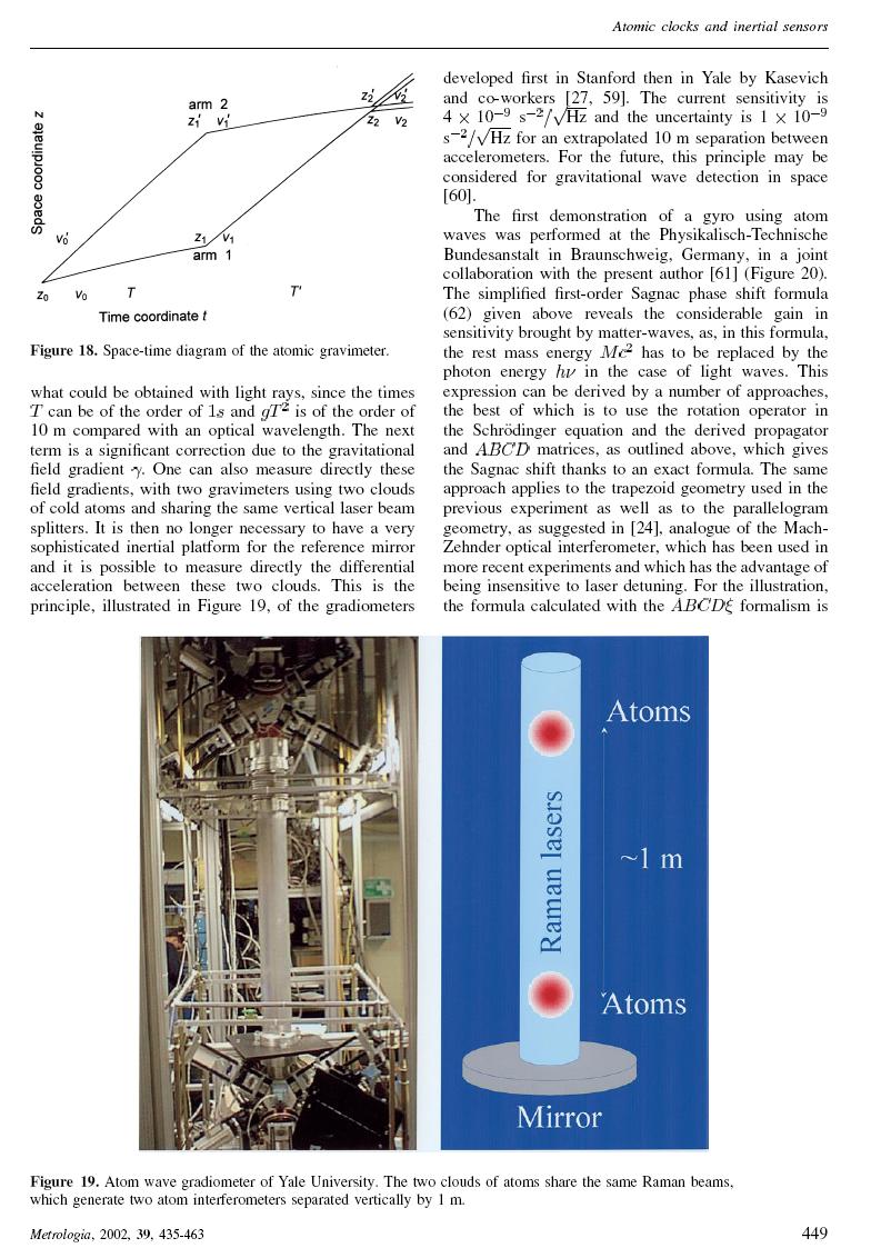
9 E(p) b a M b M a p //

10 E M ˆ p pˆ p

11 t dσ dt dx ds s τ ˆ dx dx ˆ ds dt dx x

12 CHEMIN OPTIQUE & PRINCIPE DE FERMAT ν S p dx E dt p dx dl + g p p M ν ν,,1,,3 E ν E E dt h dx (3) λdb g g p Hamilton-Jaobi g φ φ M / équation d'ionale si M ν dl f i dx i dx f i g i g i g g λ ( 3) db E g h M

13 CHEMIN OPTIQUE & PRINCIPE DE FERMAT 1 ϕ ˆϕ ϕ τ équation d'ionale à 5D ( ˆ, νˆ,1,,3, 4): g ˆ ν ˆ φ ˆ ˆ ν φ dl (4) hφ p dx ˆ E dt + dx ˆ g g dl f i (4) i fidx dx + d τ ( 4 ) g i g i g g λ h E g g

14 BASICS OF ATOM /PHOTON OPTICS Paraboli approximation of slowly varying phase and amplitude E(p) 4 E M * Massive partiles M E M + E M E(p) p p ω 3 Photons ω / 1 k p

15 BASICS OF ATOM /PHOTON OPTICS Shroedinger-like equation for the atom /photon field: * ϕ M ν i ϕ p p * + p p 4 ϕ+ p h p * νϕ t M M p i p i p M * ; 4 τ ; ( ω / for photons) - gravitation field: h g. q/ q. γ. q/ - rotation field: h α. q/ - gravitational wave: h β δ + + * * * Hext p. α( t). q p. β( t). p/ M M q. γ( t). q/ M gq. f. p

16 ABCDξφ LAW OF ATOM OPTICS + + * * * Hext p. α( t). q p. β( t). p/ M M q. γ( t). q/ M gq. f. p wavepaket ( q, t ) exp isl / exp ip ( t) q q ( t) / F q q ( t), X ( t), Y ( t) p ( p, p, p, M); q ( x, y, z, τ ) ( ) exp ip () t ( q q () t )/ F ( q q (), t X(), t Y() t ) x y z q t Aq t Bp t M t t * ( ) ( ) + ( )/ + ξ (, ) p t M Cq t Dp t M t t * * ()/ ( ) + ( )/ + φ(, ) X() t AX( t ) + BY( t ) Yt ( ) CXt ( ) + DYt ( ) Framework valid for Hamiltonians of degree in position and momentum

17 Hamilton s equations for the external motion + + * * * Hext p. α( t). q p. β( t). p/ M M q. γ( t). q/ M gq. f. p M q χ * dhext p/ M d dp χ α() t β() t f() t χ + Γ () t χ +Φ() t dt 1 dhext γ() t α() t g() t * M dq ( tt) ( ) ( ) ( ) ( ) ( ) ( ) A tt, Btt, ξ tt, χ() t χ( t ) + C t, t D t, t φ t, t ( ) ( ) t T ( ) ( ) t Att, Btt, α(') t β(') t, exp dt' C t, t D t, t γ(') t α(') t ( tt, ) ( tt, ) ξ t ( tt, ') ( t') dt' φ M Φ t

18 Laser beams Atoms Total phaseation integral+end splitting+beam splitters

19 GENERAL FORMULA FOR THE PHASE SHIFT OF AN ATOM INTERFEROMETER k β1 k β k βn β 1 M β1 β M β β N M βn βd k α1 k α k αn α 1 M α1 α M α α N M αn α D t 1 t 1 N 1 t N ( ) ( ) + 1 α + 1 δϕ Sβ t, t S t, t / N + ( k ) ( ) ( ) β qβ kα qα ωβ ωα t ϕβ ϕα ( ) ( ) + p q q p q q βd βd αd αd t D

20 The four end-points theorem β1 M β β x M α α p ( p α1 x, py, pz) q y z t 1 T t - t 1 t qβ qα qβ1 qα1 ( τβ τα) p β + p α p β1+ p α1 + Mβ + Mα ( ) ( ) ( ) ( ) ( ) Lagrange Invariant ( ) ( τ τ ) ( ) τ τ τ + τ S S M M ( M M ) ( M M ) β α β α β α ( β τβ α τα) β + α β α ( ) ( q q ) ( ) ( q q ) + p β + p α p β1+ p α1 ( Mβ Mα) β α β1 α1 β α p dx

21 GENERAL FORMULA FOR THE PHASE SHIFT OF AN ATOM/PHOTON INTERFEROMETER k β1 k β k βn β 1 M β1 β M β βn M βn βd k α1 k α k αn α 1 M α1 α M α α N M αn α D N 1 ( ) ( k ) ( q k q k k β β α α β α )( qβ qα ) δϕ + ( τβ + τα ) ( ) ω ω t ω + ϕ ϕ () β α βα β α ( ) ω () βα Mβ Mα / /

22 GENERAL FORMULA FOR THE PHASE SHIFT OF AN ATOM/PHOTON INTERFEROMETER N (5) (5) ( k. q ) 1 δϕ δ + δϕ () (5) (5) k ω ω ( kx, ky, kz, ), ; q ( x, y, z, ), t (5) (5) δ k k k ; q q + q / ( ) (5) (5) (5) (5) β α β α [ τ ]

23 Atomi Gravimeter Spae oordinat e z * v ' z 1 z 1 v 1 A( Tz)( 1 zat ( g)( / zγ ) + gb/ ( γ ) T+ ) Bp ( T/ )v M + g /γ τ * * * 1 armp / IM C( T)( z g/ γ ) + D( T) p / M + k/ M z v τ T Time oordinate t arm II z 1 ' v 1 ' τ 4 τ 3 T' z ' v ' z v * z ( ) ( ) z' M τ1+ τ3 τ τ4 + p + k+ p' 1 δϕ kz ( z z' + z) + kz ( z' )/ 1 1 p dx

24 Exat phase shift for the atom gravimeter δϕ kz ( z z' + z) + kz ( z' )/ 1 1 k sinh ( ( ')) sinh ( ) k γ T T γt + v + * γ M ( ( )) ( ) g γ + γ 1+ osh γ T + T' osh γt z whih an be written to first-order in γ, with TT : 7 k δϕ M kgt kγt gt v T z * Referene: Ch. J. B., Theoretial tools for atom optis and interferometry, C.R. Aad. Si. Paris,, Série IV, p , 1

25 ARBITRARY 3D TIME-DEPENDENT GRAVITO-INERTIAL FIELDS * * Hamiltonian: H p. α( t). q+ p. β( t). p/ M M q. γ( t). q/ Hamilton's equns: A B α β T exp dt C D γ α Example: Phase shift indued by a gravitational wave Einstein oord.: β 1+ hos ξt + φ, γ, with h h ( ) { i} ( ) h ( t ) Fermi oord.: β 1, γ ξ / os ξ + φ Einstein oord.: Fermi oord.: A 1 h B t + sin ( ξt φ) sinφ ξ + h hξ t A 1 os( ξt+ φ) osφ sinφ h ht B t+ sin ( ξt+ φ) sinφ os( ξt+ φ) + osφ ξ

26 Atomi phase shift indued by a gravitational wave δϕ khv ξ T sin ξt + φ sin ξt / khq ( ) ( ) / os T + os T + + os ( ) ( ) ξ φ ξ φ φ khv T os( T + ) os( T + ) + + ξ φ ξ φ ϕ ϕ ϕ 1 k V p + / M * Ch.J. Bordé, Gen. Rel. Grav. 36 (Marh 4) Ch.J. Bordé, J. Sharma, Ph. Tourren and Th. Damour, Theoretial approahes to laser spetrosopy in the presene of gravitational fields, J. Physique Lettres 44 (1983) L983-99

29 Bordé-Ramsey interferometers Laser beams Atom beam ( )T M M M a b b / ) ( * * * 1 + ω δϕ ( ) 1 1 * 1 k p M M b b + + ( ) 1 1 * k p M M b b + 1 * p M M a a +

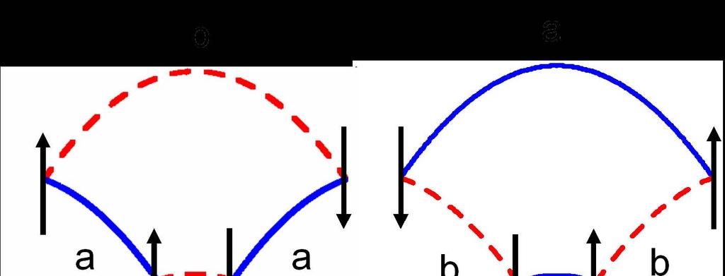
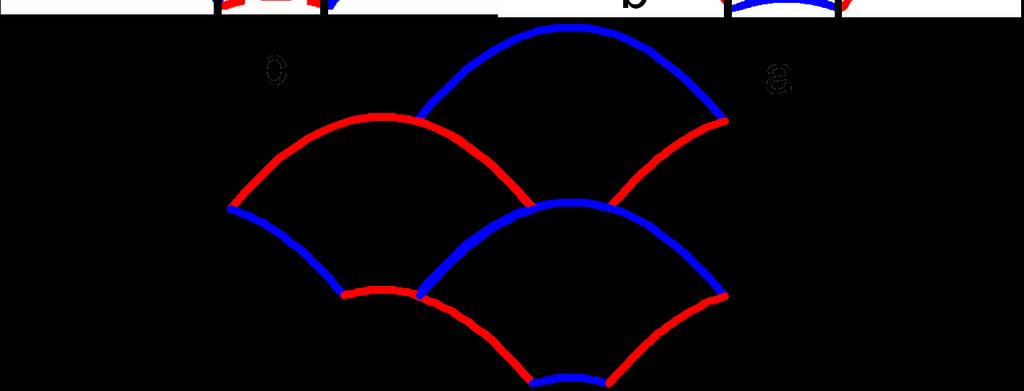
30 BORDÉ-RAMSEY INTERFEROMETERS

31 Atom Bordé-Ramsey interferometers Laser beams beam * M k T hos T + sin T * M ( ) ( ) δϕ ξ φ ξ

32 SF [ ] [ ] d dq p d X p d d x p τ τ ϕ MOLECULAR INTERFEROMETRY [ ] τ τ ϕ ˆ ˆ X d P d M X d P d d x p + +

33 What did you expet?

Σχετικά έγγραφα

Solutions - Chapter 4

Solutions - Chapter 4 Solutions - Chapter Kevin S. Huang Problem.1 Unitary: Ût = 1 ī hĥt Û tût = 1 Neglect t term: 1 + hĥ ī t 1 īhĥt = 1 + hĥ ī t ī hĥt = 1 Ĥ = Ĥ Problem. Ût = lim 1 ī ] n hĥ1t 1 ī ] hĥt... 1 ī ] hĥnt 1 ī ]