Kinematics Vs Dynamics

Transcript

1 Kinematics Vs Dynamics

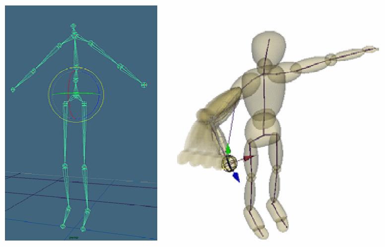
2 Kinematics Focus on articulated structures There are two ways to pose/animate an articulated character forward and inverse kinematics

3 Kinematics

4

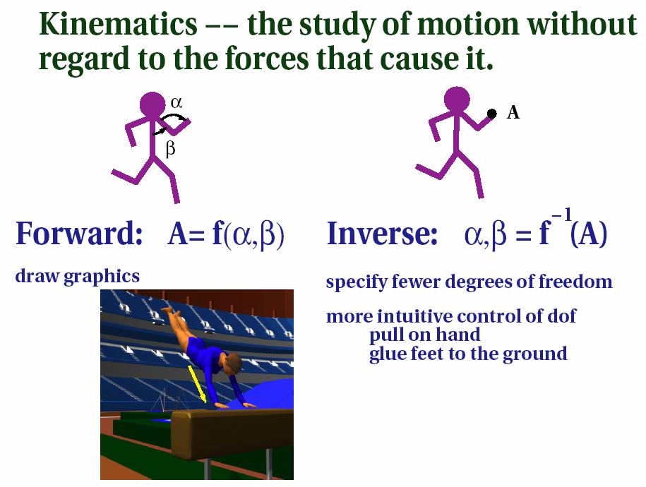
5 Forward vs. Inverse Kinematics Forward Kinematics Compute configuration (pose) given individual DOF values Keyframe animation belongs to forward kinematics Inverse Kinematics Compute individual DOF values that result in specified end effector position

6 Forward Kinematics Hierarchical model - joints and links Joints - rotational or prismatic Joints - 1, 2, or 3 Degree of Freedom Links - displayable objects Pose - setting parameters for all joint DoFs Pose Vector - a complete set of joint parameters

7

8

9 Degrees of Freedom (DOFs) The variables that affect an object s orientation How many degrees of freedom when flying? So the kinematics of this airplane permit movement anywhere in three dimensions Six x, y, and z positions roll, pitch, and yaw

10 Degrees of Freedom How about this robot arm? Five 1-base, 1-shoulder, 1-elbow, 2-wrist

11 Reachable Workspace The set of all possible positions (defined by kinematics) the end effector can reach Dextrous workspace

12 Example: 2-Link Structure

13 Forward Kinematics

14 Forward Kinematics

15 MoCap data can be used Forward Kinematics Difficult to achieve coordinated motion for articulated structures

16 Forward Kinematics

17

18

19 Drawing Articulated Figures

20 Static Figure Transformations

21 Forward Kinematics Control

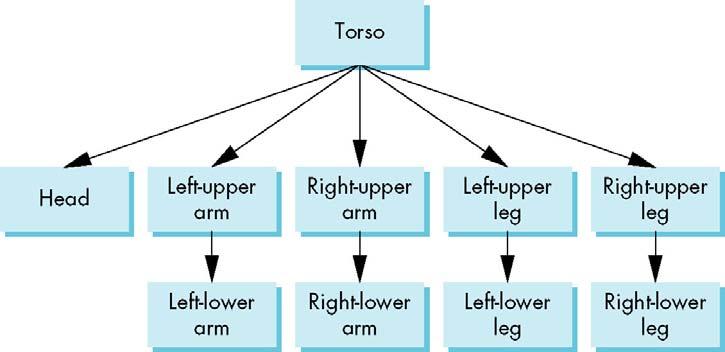
22 Hierarchy Representation All body frames are local (relative to parent) Transformations affecting root affect all children Transformations affecting any node affect all its children

23

24 Transformations at the arcs T0 T1.1 T2.1 R1.1 R2.1 T1.2 T2.2 R1.2 R2.2 User modifies Rotation (new pose vector ) Re-traverse tree To get new pose

25

26

27

28 Ροµποτικός βραχίονας Τρεις βαθµοί ελευθερίας: Γωνία περιστροφής της βάσης Γωνίες στις αρθρώσεις Μετρώνται στο σύστηµα συντεταγµένων (frame) του αντίστοιχου µέρους

29 Ροµποτικός βραχίονας Καθώς µεταβάλλονται οι γωνίες των βραχιόνων τα αντικείµενα ή τα frames τους βραχιόνων µετακινούνται ως προς τη βάση Έχει προηγηθεί τοποθέτηση στη σωστή σχετική θέση

30 Ροµποτικός βραχίονας Ηκίνηση ενός µέρους πρέπει να µεταδοθεί στα µέρη άνωθεν αυτού Περιστροφή βάσης µε πίνακα περιστροφής R y (θ) Ο κάτω βραχίονας πρέπει να περιστραφεί, να τοποθετηθεί στην κορυφή της βάσης και να περιστραφεί µαζί της: R y (θ) T(0,h 1,0) R z (φ) Ο πάνω βραχίονας πρέπει να περιστραφεί κατά ψ και να τοποθετηθεί στην κορυφή του κάτω βραχίονα: R y (θ) T(0,h 1,0) R z (φ) T(0,h 2,0) R z (ψ)

31 Ροµποτικός βραχίονας glrotate() base() gltranslate() glrotate() lower_arm() gltranslate() glrotate() upper_arm() Modelview matrix contains all transformations so far (product of transformation matrices)

32 Drawing Articulated Figure

33 ιάσχιση δένδρων ιάσχιση του δένδρου για την απεικόνιση του σύνθετου αντικειµένου Preorder διάσχιση: αναδροµική διάσχιση ρίζας, αριστερού υποδένδρου, δεξιού υποδένδρου Συνάρτηση που πραγµατοποιεί την διάσχιση Αναλυτικά µε κατάλληλη χρήση σωρών για αποθήκευση των απαιτούµενων µετασχηµατισµών Με αναδροµικό τρόπο

34 ιάσχιση δένδρων

35 Όταν µετακινούµαι σε νέο κλαδί πρέπει να επαναφέρω τον modelview (popmatrix) Όταν πάω σε παιδί ο modelview του πατέρα κληρονοµείται (επηρεάζει το παιδί) όπως θα έπρεπε

36 ιάσχιση µε βάση σωρούς Χρήση push και pop για αποµόνωση των µετασχηµατισµών glpushmatrix() torso(); gltranslate(); glrotate; Head(); glpopmatrix(); glpushmatrix() gltranslate(); glrotate; Left_upper_leg(); gltranslate(); glrotate; Left_lower_leg();

37 ιάσχιση µε βάση τους σωρούς Η µέθοδος µε τους σωρούς απαιτεί κώδικα γραµµένο για το συγκεκριµένο αντικείµενο δεν δίνει µια γενική συνάρτηση διάσχισης δένδρου.

38 ενδρικές δοµές δεδοµένων Χρήση κατάλληλων δοµών δεδοµένων (lists) για την αναπαράσταση των δένδρων και ένα γενικό αλγόριθµο διάσχισης Αναπαράσταση δένδρου: left child, right sibling Κάθε κόµβος έχει δείκτη στο αριστερότερο παιδί και στον δεξιό αδερφό (κόµβος στο ίδιο επίπεδο, παιδί του ίδιου πατέρα)

39 ενδρικές δοµές δεδοµένων

40 ενδρικές δοµές δεδοµένων Σε κάθε κόµβο αποθηκεύουµε: είκτη σε συνάρτηση που ζωγραφίζει το αντικείµενο Πίνακα µετασχηµατισµού που τοποθετεί το αντικείµενο σε σχέση µε τον πατέρα είκτες σε αριστερό παιδί, αδερφό typedef struct treenode{ GLfloat m[16]; void (*f)(); struct treenode *sibling; struct treenode *child; }treenode; ιαφορετική προσέγγιση από την προηγούµενη

41 ενδρικές δοµές δεδοµένων Κατά την απεικόνιση ο πίνακας m πολλαπλασιάζεται µε τον τρέχοντα πίνακα µετασχηµατισµού και καλείται η f Αρχικοποιούµε κατάλληλα τον κάθε κόµβο ίνουµε την αρχική θέση και την συσχέτιση µε τους υπόλοιπους κόµβους

42 ενδρικές δοµές δεδοµένων treenode torso_node, head_node, lua_node,.. glloadidentity(); glrotatef(theta[0], 0.0, 1.0, 0.0); //φτιάχνουµε κατάλληλο modelview και τον αποθηκεύουµε στον m glgetfloatv(gl_modelview_matrix,torso_node.m); torso_node.f = torso; torso_node.sibling = NULL; torso_node.child = &head_node; //Το theta είναι µεταβλητή που αλλάζει για να πετύχω την κίνηση

43 ενδρικές δοµές δεδοµένων glloadidentity(); gltranslatef(-(torso_radius+upper_arm_radius), 0.9*TORSO_HEIGHT, 0.0); //το µετακινώ στη σωστή θέση glrotatef(theta[3], 1.0, 0.0, 0.0); //µεταβλητή γωνία glgetfloatv(gl_modelview_matrix,lua_node.m); lua_node.f = left_upper_arm; lua_node.sibling = &rua_node; lua_node.child = &lla_node;

44 ενδρικές δοµές δεδοµένων Όταν µετακινούµαι σε αδερφό πρέπει να επαναφέρω τον modelview (popmatrix) Όταν πάω σε παιδί ο modelview του πατέρα κληρονοµείται όπως θα έπρεπε Αν αλλάξω τις γωνίες (DOF) ξαναδιασχίζω το δέντρο. Μπορούµε να προσθέσουµε / διαγράψουµε κόµβους δυναµικά. Αλλαγές στο αντικείµενο

45 ενδρικές δοµές δεδοµένων Αναδροµική συνάρτηση διάσχισης (preorder) Γενική, ανεξάρτητη από το συγκεκριµένο δέντρο void traverse(treenode* root){ if(root==null) return; glpushmatrix(); glmultmatrixf(root->m); root->f(); if(root->child!=null) traverse(root->child); glpopmatrix(); } if(root->sibling!=null) traverse(root->sibling);

46 Example: 2-Link Structure

47 Inverse Kinematics

48 What is Inverse Kinematics? Forward Kinematics? θ 1 θ 2 θ 3 End Effector Base r x = r f(θ)

49 What is Inverse Kinematics? Inverse Kinematics θ 1 θ2 θ3 End Effector Base r θ = r f 1 ( x)

50 Inverse Kinematics

51 Inverse Kinematics : When useful? Want character to push a button or take a step can give the animator a good first step that he/she can later fine tune

52 What Makes IK Hard? Goal of "natural looking" motion Singularities Redundancy

53 Inverse Kinematics

54 Analytical Solutions

55

56

57 r f(θ) What does looks like? l 1 l 2 θ 2 l 3? End Effector θ 1 Base θ 3 x y = = l l 1 1 cos( θ ) + 1 sin( θ ) + 1 l l 2 2 cos( θ ) sin( θ ) + l l 3 3 cos( θ ) sin( θ ) 3 3

58 Solution to r θ = r f 1 ( x) Our example x = l cos( θ ) + l cos( θ y = l sin( θ ) + 1 l ) + l sin( θ ) + l 3 3 cos( θ ) sin( θ ) Number of equations : 2 Unknown variables : 3 Infinite number of solutions! 3 3

59 Redundancy System DOF > End Effector DOF Our example x y = l = l 1 1 cos( θ ) + 1 sin( θ ) + System DOF = 3 1 l l 2 2 cos( θ ) sin( θ ) + End Effector DOF = 2 l l 3 3 cos( θ ) sin( θ ) 3 3

60 Redundancy A redundant system has infinite number of solutions Human skeleton has 70 DOF Ultra-super redundant How to solve highly redundant system?

61 IK Incremental Constructions Configurations too complex for analytical solution? Motion can be incrementally constructed At each time step, compute best way to change each joint angle to match the desired endpoint This computation forms the matrix of partial derivatives (Jacobian)

62 IK Incremental Constructions

63 IK -> Incremental Constructions w2 d2 End Effector q 2 w2 x d2 - Compute instantaneous effect of each joint - Find linear combination to take end effector towards goal position

64 IK -> Incremental Constructions

65 IK Incremental Constructions : Mathematics Unknowns End effector velocities Joint angles Approach valid for small changes

66 IK Incremental Constructions : Mathematics V vector of linear and rotational velocities represents the desired change in the end effector Unknowns (joint angle velocities) Desired change difference between current position/orientation to that specified by the goal configuration

67 Jacobian changes with time IK Incremental Constructions : Mathematics Jacobian: what is the effect of a specific joint angle change to a certain component of V

68 IK Incremental Constructions : Mathematics Rotational change ω at end effector: velocity of joint angle about the axis of revolution Linear change at end effector: cross product of axis of revolution and vector from joint to effector

69 Using the Jacobian

70 IK -> Incremental Constructions Solution only valid for an instantaneous step Once a step is taken, need to recompute solution

71 IK Incremental Constructions : Example Planar configuration We are not interested in the orientation of end effector! Axis of rotation of all joints: perpendicular to the figure

72 IK Incremental Constructions : Mathematics Jacobian: what is the effect of a specific joint angle change to a certain component of V

73 IK Incremental Constructions : Example V=g 1 θ 1 + g 2 θ 2 + g 3 θ 3

74 IK Incremental Constructions : Example Singularities No linear combination of g s will lead to the target Jacobian is not invertible

75 For redundant systems the Jacobian is not a square matrix. Use pseudoinverse (if possible)

76 Secondary goals Due to redundancy multiple solutions exist A point can be reached with many arm configurations A redundant system is more dextrous Can use redundancy and find solutions that allow e.g. obstacle avoidance or are more natural

77 Secondary goals Such a change in the DOF does not result in a change of the end effector velocities

78 Secondary goals Bias the solution towards desired angles, e.g. middle angle between joint limits (soft constraints)

79 Secondary goals Such a solution reaches both the primary goal and also is biased towards the secondary goal