2013 Aymeric Bethencourt et al., licensee Versita Sp. z o. o.
|
|
|
- Ἀναξαγόρας Λευί Σκλαβούνος
- 7 χρόνια πριν
- Προβολές:
Transcript
1 Aymeric Bethencourt et al., licensee Versita Sp. z o. o. This work is licensed under the Creative Commons Attribution-NonCommercial-NoDerivs license, which means that the text may be used for non-commercial purposes, provided credit is given to the author. Autonomous Underwater Vehicles Aymeric.Bethencourt@ensta-bretagne.fr Luc.Jaulin@ensta-bretagne.fr Kalman Filter Extended Kalman Filter Sequential Monte Carlo R R n tubes 233
2 i ẋ i = f(x i, u i ) + n x y i = g(x i ) (evolution equation) (observation equation) (1) x i i u i y i f g n x y i Formulation intertemporal relation ping p = (a, b, i, j) a R b R i {1,..., m} j {1,..., m} b > a (a, b) t p (k) k th t τ = h i (t) t τ i h i i {1,..., m} t R k {1,..., k max } (i) ẋ i (t) = f (x i (t), u i (t)) + n x (t) (ii) g ( x i(k) (a (k)), x j(k) (b (k)), a (k), b (k) ) = 0 (iii) ã (k) = h i(k) (a (k)) (iv) b (k) = h j(k) (b (k)) (v) ḣ i (t) = 1 + n h (t) (2) b(k) a(k) a(k) b(k) Simultaneous Localization and Mapping k t = a(k) t = b(k) c (b(k) a(k)) c a(k) b(k) h i n x (t) g : R n R n R R g (x 1, x 2, a, b) = x 1 x 2 c (b a) (3) c (x i(k) (a (k)) x j(k) (b (k))) 2 c (b(k) a(k)) = +(y i(k) (a (k)) y j(k) (b (k))) 2 (4) ã (k) i (k) k th b (k) j (k) k th n h (t) k ã (k), b (k), i (k), j (k). Z z Z z Z z x h lattice (E, ) x y join x y supremum meet x y 234
3 R n x y i {1,..., n}, x i y i. x y = (x 1 y 1,..., x n y n ) and x y = (x 1 y 1,..., x n y n ) x i y i = min (x i, y i ) x i y i = max (x i, y i ). E complete A E A A A E E E R R = R {, } = E = E (E 1, 1 ) (E 2, 2 ) (E, ) (a 1, a 2 ) E 1 E 2 (a 1, a 2 ) (b 1, b 2 ) ((a 1 1 b 1 ) and (a 2 2 b 2 )). interval [x] x x [x] = [x, x] = {x R, x x x} This representation has several advantages: It allows us to represent random variables with imprecise probability density functions, deal with uncertainties in a reliable way and last but foremost, it is possible to contract the interval around all feasible values given a set of constraints ( i.e. equations or inequalities). closed interval interval [x] E E [x] = {x E [x] x [x]}. E E E IE E [x] E [x] = [ [x], [x]] E. = [, ] R ; R = [, ] R ; [0, 1] R [0, ] R R {2, 3, 4, 5} = [2, 5] N N {4, 6, 8, 10} = [4, 10] 2N 2N intersection [x] [y] [x] [y] = { [max{x, y}, min{ x, ȳ}] if max{x, y} min{ x, ȳ} otherwise [1, 3] [2, 5] = [2, 3] union [x] [y] [x] [y] = [min{x, y}, max{ x, ȳ}] [1, 3] [5, 7] = [1, 7] We can apply arithmetic operators and functions to intervals to obtain all feasible values of the variable. For example, consider a real α [x] α[x] = { [αx, α x] [α x, αx ] if α 0 if α 0 [x] [y] {+,,, /} [x] [y] x y x [x] y [y] [x] [y] = [{x y R x [x], y [y]}] [x] + [y] = + y, x ȳ] [x [x] [y] = ȳ, x y] [x [x] [y] = [min{x y,x ȳ, xy, xȳ}, max{x y,x ȳ, xy, xȳ}] [1/ȳ, 1/y] 1/[y] = [1/ȳ, [ ], 1/ȳ] ], [ [x]/[y] = [x] (1/[y]) if [y] = [0, 0] if 0 / [y] if y = 0 and ȳ > 0 if y < 0 and ȳ = 0 if y < 0 and ȳ > 0 [ 1, 3] + [2, 7] = [1, 10] [ 1, 3] [2, 7] = [ 8, 1] [ 1, 3].[2, 7] = [ 7, 21] [ 1, 3]/[2, 7] = [ 1/2, 3/2] f([x]) f f([x]) = {f(x) x [x]} f f([x]) [f]([x]) = [{f(x) x [x]}] [x] [exp]([x]) = [exp x, exp x] [cos]([ π, π]) = [ 1, 1] [cos( π), cos(π)] = [ 1, 1] n x x i R, i {1,..., n f } n f f j (x 1, x 2,..., x nx ) = 0, j {1,..., n f } (5) 235 nauthent cated
4 f j x i X i [x i ] x = (x 1, x 2,..., x nx ) T x [x] = [x 1 ].[x 2 ]...[x nx ] f f j f(x) = 0 constraint satisfaction problem I I : (f(x) = 0, x [x]) S I S = {x [x] f(x) = 0} I [x] [x ] S [x ] [x] I [x] S I contractor constraint satisfaction problems I : (f(x) = 0, x [x]) f j (x 1, x 2,..., x nx ) = 0 f j +,,, /, sin, cos, exp,...etc d = (x i x j ) 2 + (y i y j ) 2 (6) i 1 = x j i 2 = x i + i 1 i 3 = i 2 2 i 4 = y j (7) i 5 = y i + i 4 i 6 = i 2 5 i 7 = i 3 + i 6 d = i 7 i k ] ; [ I d = i 7 d = i 7 i 7 = d 2 [d] = [d] [i 7 ] [i 7 ] = [i 7 ] [d 2 ] et s consider the constraint i 7 = i 3 + i 6 initial intervals [i 3 ] = [, 2], [i 6 ] = [, 3] and [i 7 ] = [4, ]. We can easily contract these intervals without removing any feasible value: i 7 = i 3 + i 6 i 7 [4, ] ([, 2] + [, 3]) = [4, ] [, 5] = [4, 5] i 3 = i 7 i 6 i 3 [, 2] ([4, ] [, 3]) = [, 2] [1, ] = [1, 2] i 6 = i 7 i 3 z [, 3] ([4, ] + [, 2]) = [, 3] [2, ] = [2, 3] We obtain much smaller intervals for [i 3 ] = [1, 2], [i 6 ] = [2, 3] and [i 7 ] = [4, 5]. tubes Tube F n R R n x y t R, x(t) y(t). tube [x] ( [x, x + ] F n x, x + t x (t) x + (t) F n IF n. x F n [x] t, x (t) [x] (t) x F 1 [x] x 236
![Algorithm C FB (in : box, inout : [x], [ẋ]) // Forward steps 1 [i 1 ] := [x j ] 2 [i 2 ] := [x i ] + [i 1 ] 3 [i 3 ] := [i 2 2 ] 4 [i 4 ] := [ y j ] 5 [i 5 ] := [y i ] + [i 4 ] 6 [i 6 ] := [i 2 5 ] 7](/docs-images/75/72656936/images/5-0.jpg "[i 7 ] := [i 3 ] + [i 6 ] 8 [d] := [d] [i 7 ] // Bacward steps 9 [i 7 ] := [i 7 ] [d] 2 10 [i 3 ] := [i 3 ] ([i 7 ] [i 6 ]) 11 [i 6 ] := [i 6 ] ([i 7 ] [i 3 ]) 12 [i 5 ] := [i 5 ] (sqr 1 [i 6 ]) 13")
5 Algorithm C FB (in : box, inout : [x], [ẋ]) // Forward steps 1 [i 1 ] := [x j ] 2 [i 2 ] := [x i ] + [i 1 ] 3 [i 3 ] := [i 2 2 ] 4 [i 4 ] := [ y j ] 5 [i 5 ] := [y i ] + [i 4 ] 6 [i 6 ] := [i 2 5 ] 7 [i 7 ] := [i 3 ] + [i 6 ] 8 [d] := [d] [i 7 ] // Bacward steps 9 [i 7 ] := [i 7 ] [d] 2 10 [i 3 ] := [i 3 ] ([i 7 ] [i 6 ]) 11 [i 6 ] := [i 6 ] ([i 7 ] [i 3 ]) 12 [i 5 ] := [i 5 ] (sqr 1 [i 6 ]) 13 [y i ] := [y i ] ([i 5 ] [i 4 ]) 14 [i 4 ] := [i 4 ] ([i 5 ] [y]) 15 [y j ] := [y j ] [i 4 ] 16 [i 2 ] := [i 2 ] (sqr 1 [i 3 ]) 17 [x i ] := [x i ] ([i 2 ] [i 1 ]) 18 [i 4 ] := [i 4 ] ([i 2 ] [x i ]) 19 [x j ] := [x j ] [i 1 ] [x] ([t]) [x] (t), t [t] x [x], t [t] x (t) [x] ([t]), [x] ([t]) Tube arithmetic F n t F n Integral., t 2 t 2 0 [x] [, t 2 ] t2 [x] (τ) dτ = { t2 } x (τ) dτ such that x [x]. t 2 t2 [ t2 t2 ] [x] (τ) dτ = x (τ) dτ, x + (τ) dτ. x [x] t2 x (τ) dτ t2 [x] (τ) dτ. interval primitive t [x] (τ) dτ 0 t = 0 Tube contractor L(x) L C L [x] [y] [x] [y] [x] R x Interval evaluation of a tube x R R n x F n x ([t]) = {x (t), t [t]}. [x] [x] ([t]) = t [t] [x] (t), ( t, [x](t) ) [y](t) (contraction) L(x) = x [y] (completeness) x [x] C minimal contractor L [y] L Minimal tube contractor L(x 1,..., x p ) x 1,..., x p IF n p x 1 = f 1 (x 2,..., x p ) x 2 = f 2 (x 1, x 3,..., x p )... Proposition 1. x y t [0, [, x(t) y(t) 237
6 x [x] y [y], C ( ) ( ) [x] [x, x + y + ] = [y] [x y, y + ] Proof. x y a y = x + a a 0 [y] = [y] ([x] + [a]) [y] = [y (x + a ), y + (x + + a + )] [y] = [y (x + 0), y + (x + + )] [y] = [y x, y + ] Proposition 3. t [0, [, x(t) = y(t T ) [a] = [0, [ x = y + a a 0 [x] = [x, x + y + ] Proposition 2. x = y t [0, [, x(t) = y(t) ( ) ( ) [x] [x y, x + y + ] C = = [y] [x y, x + y + ] Proof. x = y x y y [x] = [x] [y] [x] = [x y, x + y + ] C delay ( ) ( ) [x] [x (t) y (t τ), x + (t) y + (t τ)] = [y] [x (t + τ) y (t), x + (t + τ) y + (t)] Proof. [x (t) y (t τ), x + (t) y + (t τ)] j [x j ] [h j ] 238
 = [x j ](t) [h j ] (t) = [h j ] (t) t 0 t 0 ([f]([u j (τ)],[x j (τ)]) + [n x (τ)])dτ (8) (1 + [n h ] (τ))dτ (9) t [x j ] [h j ] [x j ] [h j ] i j [x i ]](/docs-images/75/72656936/images/7-0.jpg "[a(k)] i k j i j [a (k)] [b(k)] [x i(k) ](a (k)) [x j(k) ](b (k)) [y i(k) ](a (k)) [y j(k) ] (b (k)) x j(k) (b (k))) [x j(k) ] ([b (k))]) (before) [x i ] [x j(k)")
![] ([b (k))]) (after) [c (b(k) a (k))] [b(k)] ẋ i (t) = ( ) ui1 (t). cos(u i2 (t)) + n x (t) u i1 (t).](/docs-images/75/72656936/images/7-1.jpg "sin(u i2 (t)) u i1 (t) u i2 (t) u i (t) i x i x i y i i n x (t) ( ) sin t x 1 (t) = 10 cos t ( ) sin(t + π) x 2 (t) = 10 cos(t + π) For AUV 1, n x (t) = 0.")
7 [x j ](t) = [x j ](t) [h j ] (t) = [h j ] (t) t 0 t 0 ([f]([u j (τ)],[x j (τ)]) + [n x (τ)])dτ (8) (1 + [n h ] (τ))dτ (9) t [x j ] [h j ] [x j ] [h j ] i j [x i ] [a(k)] i k j i j [a (k)] [b(k)] [x i(k) ](a (k)) [x j(k) ](b (k)) [y i(k) ](a (k)) [y j(k) ] (b (k)) x j(k) (b (k))) [x j(k) ] ([b (k))]) (before) [x i ] [x j(k) ] ([b (k))]) (after) [c (b(k) a (k))] [b(k)] ẋ i (t) = ( ) ui1 (t). cos(u i2 (t)) + n x (t) u i1 (t). sin(u i2 (t)) u i1 (t) u i2 (t) u i (t) i x i x i y i i n x (t) ( ) sin t x 1 (t) = 10 cos t ( ) sin(t + π) x 2 (t) = 10 cos(t + π) For AUV 1, n x (t) = 0.1t and n h (t) = 0.01t For AUV 2, n x (t) = t and n h (t) = 0.1t 239
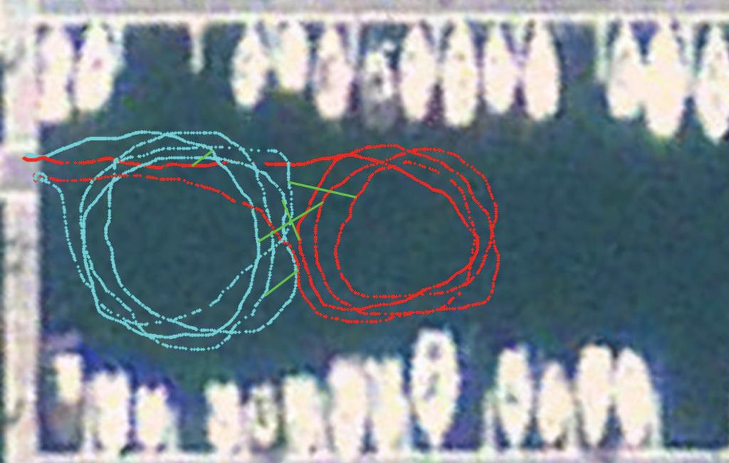
 τ = h(t) (10, 0) T ( 10, 0) T c = 100 k = 0 t = 1 ã(0) = 1 a(0) [h 1 ] [a(0)] [x 1 ] [y 1 ] [x 1 ]([a(0)]) [y 1 ]([a(0)]) ã(0) [a(0)] [x 1 ]([a(0)]) [y 1 ]([a(0)]) 1.00 [0.99, 1.01] [5.21, 5.](/docs-images/75/72656936/images/8-1.jpg "59] [8.26, 8.57] t = 1.37 b(0) = 1.37 b(0) [h 2 ] [b(0)] [x 2 ] [y 2 ] [x 2 ]([b(0)]) [y 2 ]([b(0)]) b(0) [b(0)] [x 2 ]([b(0)]) [y 2 ]([b(0)]) 1.37 [1.22, 1.51] [ 4.67, 0.90] [ 11.49, 8.")
8 [h](t) τ = h(t) (10, 0) T ( 10, 0) T c = 100 k = 0 t = 1 ã(0) = 1 a(0) [h 1 ] [a(0)] [x 1 ] [y 1 ] [x 1 ]([a(0)]) [y 1 ]([a(0)]) ã(0) [a(0)] [x 1 ]([a(0)]) [y 1 ]([a(0)]) 1.00 [0.99, 1.01] [5.21, 5.59] [8.26, 8.57] t = 1.37 b(0) = 1.37 b(0) [h 2 ] [b(0)] [x 2 ] [y 2 ] [x 2 ]([b(0)]) [y 2 ]([b(0)]) b(0) [b(0)] [x 2 ]([b(0)]) [y 2 ]([b(0)]) 1.37 [1.22, 1.51] [ 4.67, 0.90] [ 11.49, 8.16] b(0) [b(0)] [x 2 ]([b(0)]) [y 2 ]([b(0)]) 1.23 [1.22, 1.23] [ 4.67, 1.25] [ 11.49, 9.98] ( ) sin t 10 i {1, 2, 3}, x i (t) = 10 cos t ( ) sin t i {4, 5, 6}, x i (t) = 10 cos t 5m 10 i = 1, 2 3 x i (t) < 9m 4,
![[h 4 ] [x](/docs-images/75/72656936/images/9-1.jpg "4 ]")

9 [h 4 ] [x 4 ] CISCREA u i
, RIO DE NOLCOS 2010 Proceedings of the International Conference on Logic Programming International Journal of Advanced Robotic Systems")
10 References IBEX Automatica Proc. CP, Constraint Programming Automatica IN PROC. 10TH INTERNATIONAL SYMPOSIUM ON EXPERIMENTAL ROBOTICS (ISER), RIO DE NOLCOS 2010 Proceedings of the International Conference on Logic Programming International Journal of Advanced Robotic Systems Méthodes ensemblistes pour le diagnostic, l estimation d état et la fusion de données temporelles. Artificial Intelligence and Symbolic Computation Artificial Intelligence Introduction to Lattices and Order ION GNSS Int. Symposium on Information Theory and its Applications IEEE Transaction on Robotics Springer-Verlag Ellipsoidal Calculus for Estimation and Control International Journal of Robotics Research Intelligent Robots and Systems, (IROS 2005)
11 IEEE/RSJ International Conference on IEEE Transactions on Automatic Systems Bounding Approaches to System Identification Methods and Applications of Interval Analysis LAP Academic Publishers, Kln, Germany Journal of the Association for Computing Machinery Probabilistic Robotics The Psychology of Computer Vision Journal of Marine Science and Application 243
![0SQ_\O [x1 ] [y1 ] b (0) [h2 ] a (0) [h2 ] [h1 ] [x2 ] [y2 ] [a(0)] [a(0)] [y1(0)]([a(0)]) [x1(0)]([a(0)]) [b(0)] [x2](/docs-images/75/72656936/images/12-0.jpg "] [b(0)] [y2(0)]([b(0)]) 244 Unauthenticated 86.72.182.150 [y2 ] [x2(0)]([b(0)]) :+6+.")
12 0SQ_\O [x1 ] [y1 ] b (0) [h2 ] a (0) [h2 ] [h1 ] [x2 ] [y2 ] [a(0)] [a(0)] [y1(0)]([a(0)]) [x1(0)]([a(0)]) [b(0)] [x2 ] [b(0)] [y2(0)]([b(0)]) 244 Unauthenticated [y2 ] [x2(0)]([b(0)]) :+6+.C8 4Y_\XKV YP,ORK`SY\KV <YLY^SM]
Generating Set of the Complete Semigroups of Binary Relations
 Applied Mathematics 06 7 98-07 Published Online January 06 in SciRes http://wwwscirporg/journal/am http://dxdoiorg/036/am067009 Generating Set of the Complete Semigroups of Binary Relations Yasha iasamidze
The challenges of non-stable predicates
 The challenges of non-stable predicates Consider a non-stable predicate Φ encoding, say, a safety property. We want to determine whether Φ holds for our program. The challenges of non-stable predicates
Schedulability Analysis Algorithm for Timing Constraint Workflow Models
 CIMS Vol.8No.72002pp.527-532 ( 100084) Petri Petri F270.7 A Schedulability Analysis Algorithm for Timing Constraint Workflow Models Li Huifang and Fan Yushun (Department of Automation, Tsinghua University,
Chapter 6: Systems of Linear Differential. be continuous functions on the interval
 Chapter 6: Systems of Linear Differential Equations Let a (t), a 2 (t),..., a nn (t), b (t), b 2 (t),..., b n (t) be continuous functions on the interval I. The system of n first-order differential equations
C.S. 430 Assignment 6, Sample Solutions
 C.S. 430 Assignment 6, Sample Solutions Paul Liu November 15, 2007 Note that these are sample solutions only; in many cases there were many acceptable answers. 1 Reynolds Problem 10.1 1.1 Normal-order
derivation of the Laplacian from rectangular to spherical coordinates
 derivation of the Laplacian from rectangular to spherical coordinates swapnizzle 03-03- :5:43 We begin by recognizing the familiar conversion from rectangular to spherical coordinates (note that φ is used
Optimization, PSO) DE [1, 2, 3, 4] PSO [5, 6, 7, 8, 9, 10, 11] (P)
![Optimization, PSO) DE [1, 2, 3, 4] PSO [5, 6, 7, 8, 9, 10, 11] (P)](/thumbs/85/92153760.jpg "Optimization, PSO) DE [1, 2, 3, 4] PSO [5, 6, 7, 8, 9, 10, 11] (P)") ( ) 1 ( ) : : (Differential Evolution, DE) (Particle Swarm Optimization, PSO) DE [1, 2, 3, 4] PSO [5, 6, 7, 8, 9, 10, 11] 2 2.1 (P) (P ) minimize f(x) subject to g j (x) 0, j = 1,..., q h j (x) = 0, j
( ) 1 ( ) : : (Differential Evolution, DE) (Particle Swarm Optimization, PSO) DE [1, 2, 3, 4] PSO [5, 6, 7, 8, 9, 10, 11] 2 2.1 (P) (P ) minimize f(x) subject to g j (x) 0, j = 1,..., q h j (x) = 0, j
Probabilistic Approach to Robust Optimization
 Probabilistic Approach to Robust Optimization Akiko Takeda Department of Mathematical & Computing Sciences Graduate School of Information Science and Engineering Tokyo Institute of Technology Tokyo 52-8552,
A Lambda Model Characterizing Computational Behaviours of Terms
 A Lambda Model Characterizing Computational Behaviours of Terms joint paper with Silvia Ghilezan RPC 01, Sendai, October 26, 2001 1 Plan of the talk normalization properties inverse limit model Stone dualities
Partial Differential Equations in Biology The boundary element method. March 26, 2013
 The boundary element method March 26, 203 Introduction and notation The problem: u = f in D R d u = ϕ in Γ D u n = g on Γ N, where D = Γ D Γ N, Γ D Γ N = (possibly, Γ D = [Neumann problem] or Γ N = [Dirichlet
Matrices and Determinants
 Matrices and Determinants SUBJECTIVE PROBLEMS: Q 1. For what value of k do the following system of equations possess a non-trivial (i.e., not all zero) solution over the set of rationals Q? x + ky + 3z
Estimation of stability region for a class of switched linear systems with multiple equilibrium points
 29 4 2012 4 1000 8152(2012)04 0409 06 Control Theory & Applications Vol 29 No 4 Apr 2012 12 1 (1 250061; 2 250353) ; ; ; TP273 A Estimation of stability region for a class of switched linear systems with
Numerical Analysis FMN011
 Numerical Analysis FMN011 Carmen Arévalo Lund University carmen@maths.lth.se Lecture 12 Periodic data A function g has period P if g(x + P ) = g(x) Model: Trigonometric polynomial of order M T M (x) =
Second Order Partial Differential Equations
 Chapter 7 Second Order Partial Differential Equations 7.1 Introduction A second order linear PDE in two independent variables (x, y Ω can be written as A(x, y u x + B(x, y u xy + C(x, y u u u + D(x, y
Chapter 6: Systems of Linear Differential. be continuous functions on the interval
 Chapter 6: Systems of Linear Differential Equations Let a (t), a 2 (t),..., a nn (t), b (t), b 2 (t),..., b n (t) be continuous functions on the interval I. The system of n first-order differential equations
k A = [k, k]( )[a 1, a 2 ] = [ka 1,ka 2 ] 4For the division of two intervals of confidence in R +
[a 1, a 2 ] = [ka 1,ka 2 ] 4For the division of two intervals of confidence in R +](/thumbs/73/69566903.jpg "k A = [k, k]( )[a 1, a 2 ] = [ka 1,ka 2 ] 4For the division of two intervals of confidence in R +") Chapter 3. Fuzzy Arithmetic 3- Fuzzy arithmetic: ~Addition(+) and subtraction (-): Let A = [a and B = [b, b in R If x [a and y [b, b than x+y [a +b +b Symbolically,we write A(+)B = [a (+)[b, b = [a +b
Chapter 3. Fuzzy Arithmetic 3- Fuzzy arithmetic: ~Addition(+) and subtraction (-): Let A = [a and B = [b, b in R If x [a and y [b, b than x+y [a +b +b Symbolically,we write A(+)B = [a (+)[b, b = [a +b
Απόκριση σε Μοναδιαία Ωστική Δύναμη (Unit Impulse) Απόκριση σε Δυνάμεις Αυθαίρετα Μεταβαλλόμενες με το Χρόνο. Απόστολος Σ.
 Απόκριση σε Δυνάμεις Αυθαίρετα Μεταβαλλόμενες με το Χρόνο. Απόστολος Σ.") Απόκριση σε Δυνάμεις Αυθαίρετα Μεταβαλλόμενες με το Χρόνο The time integral of a force is referred to as impulse, is determined by and is obtained from: Newton s 2 nd Law of motion states that the action
Απόκριση σε Δυνάμεις Αυθαίρετα Μεταβαλλόμενες με το Χρόνο The time integral of a force is referred to as impulse, is determined by and is obtained from: Newton s 2 nd Law of motion states that the action
Lecture 2: Dirac notation and a review of linear algebra Read Sakurai chapter 1, Baym chatper 3
 Lecture 2: Dirac notation and a review of linear algebra Read Sakurai chapter 1, Baym chatper 3 1 State vector space and the dual space Space of wavefunctions The space of wavefunctions is the set of all
A Two-Sided Laplace Inversion Algorithm with Computable Error Bounds and Its Applications in Financial Engineering
 Electronic Companion A Two-Sie Laplace Inversion Algorithm with Computable Error Bouns an Its Applications in Financial Engineering Ning Cai, S. G. Kou, Zongjian Liu HKUST an Columbia University Appenix
Statistics 104: Quantitative Methods for Economics Formula and Theorem Review
 Harvard College Statistics 104: Quantitative Methods for Economics Formula and Theorem Review Tommy MacWilliam, 13 tmacwilliam@college.harvard.edu March 10, 2011 Contents 1 Introduction to Data 5 1.1 Sample
Other Test Constructions: Likelihood Ratio & Bayes Tests
 Other Test Constructions: Likelihood Ratio & Bayes Tests Side-Note: So far we have seen a few approaches for creating tests such as Neyman-Pearson Lemma ( most powerful tests of H 0 : θ = θ 0 vs H 1 :
Adaptive grouping difference variation wolf pack algorithm
 3 2017 5 ( ) Journal of East China Normal University (Natural Science) No. 3 May 2017 : 1000-5641(2017)03-0078-09, (, 163318) :,,.,,,,.,,. : ; ; ; : TP301.6 : A DOI: 10.3969/j.issn.1000-5641.2017.03.008
CHAPTER 25 SOLVING EQUATIONS BY ITERATIVE METHODS
 CHAPTER 5 SOLVING EQUATIONS BY ITERATIVE METHODS EXERCISE 104 Page 8 1. Find the positive root of the equation x + 3x 5 = 0, correct to 3 significant figures, using the method of bisection. Let f(x) =
The Simply Typed Lambda Calculus
 Type Inference Instead of writing type annotations, can we use an algorithm to infer what the type annotations should be? That depends on the type system. For simple type systems the answer is yes, and
EE512: Error Control Coding
 EE512: Error Control Coding Solution for Assignment on Finite Fields February 16, 2007 1. (a) Addition and Multiplication tables for GF (5) and GF (7) are shown in Tables 1 and 2. + 0 1 2 3 4 0 0 1 2 3
Section 8.3 Trigonometric Equations
 99 Section 8. Trigonometric Equations Objective 1: Solve Equations Involving One Trigonometric Function. In this section and the next, we will exple how to solving equations involving trigonometric functions.
ST5224: Advanced Statistical Theory II
 ST5224: Advanced Statistical Theory II 2014/2015: Semester II Tutorial 7 1. Let X be a sample from a population P and consider testing hypotheses H 0 : P = P 0 versus H 1 : P = P 1, where P j is a known
6.3 Forecasting ARMA processes
 122 CHAPTER 6. ARMA MODELS 6.3 Forecasting ARMA processes The purpose of forecasting is to predict future values of a TS based on the data collected to the present. In this section we will discuss a linear
Example Sheet 3 Solutions
 Example Sheet 3 Solutions. i Regular Sturm-Liouville. ii Singular Sturm-Liouville mixed boundary conditions. iii Not Sturm-Liouville ODE is not in Sturm-Liouville form. iv Regular Sturm-Liouville note
Statistical Inference I Locally most powerful tests
 Statistical Inference I Locally most powerful tests Shirsendu Mukherjee Department of Statistics, Asutosh College, Kolkata, India. shirsendu st@yahoo.co.in So far we have treated the testing of one-sided
D Alembert s Solution to the Wave Equation
 D Alembert s Solution to the Wave Equation MATH 467 Partial Differential Equations J. Robert Buchanan Department of Mathematics Fall 2018 Objectives In this lesson we will learn: a change of variable technique
Phys460.nb Solution for the t-dependent Schrodinger s equation How did we find the solution? (not required)
") Phys460.nb 81 ψ n (t) is still the (same) eigenstate of H But for tdependent H. The answer is NO. 5.5.5. Solution for the tdependent Schrodinger s equation If we assume that at time t 0, the electron starts
Phys460.nb 81 ψ n (t) is still the (same) eigenstate of H But for tdependent H. The answer is NO. 5.5.5. Solution for the tdependent Schrodinger s equation If we assume that at time t 0, the electron starts
3.4 SUM AND DIFFERENCE FORMULAS. NOTE: cos(α+β) cos α + cos β cos(α-β) cos α -cos β
 cos α + cos β cos(α-β) cos α -cos β") 3.4 SUM AND DIFFERENCE FORMULAS Page Theorem cos(αβ cos α cos β -sin α cos(α-β cos α cos β sin α NOTE: cos(αβ cos α cos β cos(α-β cos α -cos β Proof of cos(α-β cos α cos β sin α Let s use a unit circle
3.4 SUM AND DIFFERENCE FORMULAS Page Theorem cos(αβ cos α cos β -sin α cos(α-β cos α cos β sin α NOTE: cos(αβ cos α cos β cos(α-β cos α -cos β Proof of cos(α-β cos α cos β sin α Let s use a unit circle
Spherical Coordinates
 Spherical Coordinates MATH 311, Calculus III J. Robert Buchanan Department of Mathematics Fall 2011 Spherical Coordinates Another means of locating points in three-dimensional space is known as the spherical
Homomorphism in Intuitionistic Fuzzy Automata
 International Journal of Fuzzy Mathematics Systems. ISSN 2248-9940 Volume 3, Number 1 (2013), pp. 39-45 Research India Publications http://www.ripublication.com/ijfms.htm Homomorphism in Intuitionistic
SOLUTIONS TO MATH38181 EXTREME VALUES AND FINANCIAL RISK EXAM
 SOLUTIONS TO MATH38181 EXTREME VALUES AND FINANCIAL RISK EXAM Solutions to Question 1 a) The cumulative distribution function of T conditional on N n is Pr T t N n) Pr max X 1,..., X N ) t N n) Pr max
SCITECH Volume 13, Issue 2 RESEARCH ORGANISATION Published online: March 29, 2018
 Journal of rogressive Research in Mathematics(JRM) ISSN: 2395-028 SCITECH Volume 3, Issue 2 RESEARCH ORGANISATION ublished online: March 29, 208 Journal of rogressive Research in Mathematics www.scitecresearch.com/journals
Solution Series 9. i=1 x i and i=1 x i.
 Lecturer: Prof. Dr. Mete SONER Coordinator: Yilin WANG Solution Series 9 Q1. Let α, β >, the p.d.f. of a beta distribution with parameters α and β is { Γ(α+β) Γ(α)Γ(β) f(x α, β) xα 1 (1 x) β 1 for < x
Real time mobile robot control with a multiresolution map representation
 IIC 06 21 Real time mobile robot control with a multiresolution map representation Katsuya Iwata, Shinkichi Inagaki, Yusuke Nara, Tatsuya Suzuki (Nagoya University) Abstract In this paper a real-time path
Inverse trigonometric functions & General Solution of Trigonometric Equations. ------------------ ----------------------------- -----------------
 Inverse trigonometric functions & General Solution of Trigonometric Equations. 1. Sin ( ) = a) b) c) d) Ans b. Solution : Method 1. Ans a: 17 > 1 a) is rejected. w.k.t Sin ( sin ) = d is rejected. If sin
Second Order RLC Filters
 ECEN 60 Circuits/Electronics Spring 007-0-07 P. Mathys Second Order RLC Filters RLC Lowpass Filter A passive RLC lowpass filter (LPF) circuit is shown in the following schematic. R L C v O (t) Using phasor
2016 IEEE/ACM International Conference on Mobile Software Engineering and Systems
 2016 IEEE/ACM International Conference on Mobile Software Engineering and Systems Multiple User Interfaces MobileSoft'16, Multi-User Experience (MUX) S1: Insourcing S2: Outsourcing S3: Responsive design
Main source: "Discrete-time systems and computer control" by Α. ΣΚΟΔΡΑΣ ΨΗΦΙΑΚΟΣ ΕΛΕΓΧΟΣ ΔΙΑΛΕΞΗ 4 ΔΙΑΦΑΝΕΙΑ 1
 Main source: "Discrete-time systems and computer control" by Α. ΣΚΟΔΡΑΣ ΨΗΦΙΑΚΟΣ ΕΛΕΓΧΟΣ ΔΙΑΛΕΞΗ 4 ΔΙΑΦΑΝΕΙΑ 1 A Brief History of Sampling Research 1915 - Edmund Taylor Whittaker (1873-1956) devised a
: Monte Carlo EM 313, Louis (1982) EM, EM Newton-Raphson, /. EM, 2 Monte Carlo EM Newton-Raphson, Monte Carlo EM, Monte Carlo EM, /. 3, Monte Carlo EM
 EM, EM Newton-Raphson, /. EM, 2 Monte Carlo EM Newton-Raphson, Monte Carlo EM, Monte Carlo EM, /. 3, Monte Carlo EM") 2008 6 Chinese Journal of Applied Probability and Statistics Vol.24 No.3 Jun. 2008 Monte Carlo EM 1,2 ( 1,, 200241; 2,, 310018) EM, E,,. Monte Carlo EM, EM E Monte Carlo,. EM, Monte Carlo EM,,,,. Newton-Raphson.
2008 6 Chinese Journal of Applied Probability and Statistics Vol.24 No.3 Jun. 2008 Monte Carlo EM 1,2 ( 1,, 200241; 2,, 310018) EM, E,,. Monte Carlo EM, EM E Monte Carlo,. EM, Monte Carlo EM,,,,. Newton-Raphson.
A Bonus-Malus System as a Markov Set-Chain. Małgorzata Niemiec Warsaw School of Economics Institute of Econometrics
 A Bonus-Malus System as a Markov Set-Chain Małgorzata Niemiec Warsaw School of Economics Institute of Econometrics Contents 1. Markov set-chain 2. Model of bonus-malus system 3. Example 4. Conclusions
Exercises 10. Find a fundamental matrix of the given system of equations. Also find the fundamental matrix Φ(t) satisfying Φ(0) = I. 1.
 satisfying Φ(0) = I. 1.") Exercises 0 More exercises are available in Elementary Differential Equations. If you have a problem to solve any of them, feel free to come to office hour. Problem Find a fundamental matrix of the given
Exercises 0 More exercises are available in Elementary Differential Equations. If you have a problem to solve any of them, feel free to come to office hour. Problem Find a fundamental matrix of the given
Finite Field Problems: Solutions
 Finite Field Problems: Solutions 1. Let f = x 2 +1 Z 11 [x] and let F = Z 11 [x]/(f), a field. Let Solution: F =11 2 = 121, so F = 121 1 = 120. The possible orders are the divisors of 120. Solution: The
Uniform Convergence of Fourier Series Michael Taylor
 Uniform Convergence of Fourier Series Michael Taylor Given f L 1 T 1 ), we consider the partial sums of the Fourier series of f: N 1) S N fθ) = ˆfk)e ikθ. k= N A calculation gives the Dirichlet formula
ECE 308 SIGNALS AND SYSTEMS FALL 2017 Answers to selected problems on prior years examinations
 ECE 308 SIGNALS AND SYSTEMS FALL 07 Answers to selected problems on prior years examinations Answers to problems on Midterm Examination #, Spring 009. x(t) = r(t + ) r(t ) u(t ) r(t ) + r(t 3) + u(t +
Congruence Classes of Invertible Matrices of Order 3 over F 2
 International Journal of Algebra, Vol. 8, 24, no. 5, 239-246 HIKARI Ltd, www.m-hikari.com http://dx.doi.org/.2988/ija.24.422 Congruence Classes of Invertible Matrices of Order 3 over F 2 Ligong An and
Homomorphism of Intuitionistic Fuzzy Groups
 International Mathematical Forum, Vol. 6, 20, no. 64, 369-378 Homomorphism o Intuitionistic Fuzz Groups P. K. Sharma Department o Mathematics, D..V. College Jalandhar Cit, Punjab, India pksharma@davjalandhar.com
Pg The perimeter is P = 3x The area of a triangle is. where b is the base, h is the height. In our case b = x, then the area is
 Pg. 9. The perimeter is P = The area of a triangle is A = bh where b is the base, h is the height 0 h= btan 60 = b = b In our case b =, then the area is A = = 0. By Pythagorean theorem a + a = d a a =
Homework 3 Solutions
 Homework 3 Solutions Igor Yanovsky (Math 151A TA) Problem 1: Compute the absolute error and relative error in approximations of p by p. (Use calculator!) a) p π, p 22/7; b) p π, p 3.141. Solution: For
6.1. Dirac Equation. Hamiltonian. Dirac Eq.
 6.1. Dirac Equation Ref: M.Kaku, Quantum Field Theory, Oxford Univ Press (1993) η μν = η μν = diag(1, -1, -1, -1) p 0 = p 0 p = p i = -p i p μ p μ = p 0 p 0 + p i p i = E c 2 - p 2 = (m c) 2 H = c p 2
2 Composition. Invertible Mappings
 Arkansas Tech University MATH 4033: Elementary Modern Algebra Dr. Marcel B. Finan Composition. Invertible Mappings In this section we discuss two procedures for creating new mappings from old ones, namely,
Matrices and vectors. Matrix and vector. a 11 a 12 a 1n a 21 a 22 a 2n A = b 1 b 2. b m. R m n, b = = ( a ij. a m1 a m2 a mn. def
 Matrices and vectors Matrix and vector a 11 a 12 a 1n a 21 a 22 a 2n A = a m1 a m2 a mn def = ( a ij ) R m n, b = b 1 b 2 b m Rm Matrix and vectors in linear equations: example E 1 : x 1 + x 2 + 3x 4 =
Probability and Random Processes (Part II)
") Probability and Random Processes (Part II) 1. If the variance σ x of d(n) = x(n) x(n 1) is one-tenth the variance σ x of a stationary zero-mean discrete-time signal x(n), then the normalized autocorrelation
Probability and Random Processes (Part II) 1. If the variance σ x of d(n) = x(n) x(n 1) is one-tenth the variance σ x of a stationary zero-mean discrete-time signal x(n), then the normalized autocorrelation
Test Data Management in Practice
 Problems, Concepts, and the Swisscom Test Data Organizer Do you have issues with your legal and compliance department because test environments contain sensitive data outsourcing partners must not see?
Lecture 2. Soundness and completeness of propositional logic
 Lecture 2 Soundness and completeness of propositional logic February 9, 2004 1 Overview Review of natural deduction. Soundness and completeness. Semantics of propositional formulas. Soundness proof. Completeness
Homework 8 Model Solution Section
 MATH 004 Homework Solution Homework 8 Model Solution Section 14.5 14.6. 14.5. Use the Chain Rule to find dz where z cosx + 4y), x 5t 4, y 1 t. dz dx + dy y sinx + 4y)0t + 4) sinx + 4y) 1t ) 0t + 4t ) sinx
Reminders: linear functions
 Reminders: linear functions Let U and V be vector spaces over the same field F. Definition A function f : U V is linear if for every u 1, u 2 U, f (u 1 + u 2 ) = f (u 1 ) + f (u 2 ), and for every u U
ΔΙΕΡΕΥΝΗΣΗ ΤΗΣ ΣΕΞΟΥΑΛΙΚΗΣ ΔΡΑΣΤΗΡΙΟΤΗΤΑΣ ΤΩΝ ΓΥΝΑΙΚΩΝ ΚΑΤΑ ΤΗ ΔΙΑΡΚΕΙΑ ΤΗΣ ΕΓΚΥΜΟΣΥΝΗΣ ΤΕΧΝΟΛΟΓΙΚΟ ΠΑΝΕΠΙΣΤΗΜΙΟ ΚΥΠΡΟΥ ΣΧΟΛΗ ΕΠΙΣΤΗΜΩΝ ΥΓΕΙΑΣ
 ΤΕΧΝΟΛΟΓΙΚΟ ΠΑΝΕΠΙΣΤΗΜΙΟ ΚΥΠΡΟΥ ΣΧΟΛΗ ΕΠΙΣΤΗΜΩΝ ΥΓΕΙΑΣ Πτυχιακή Εργασία ΔΙΕΡΕΥΝΗΣΗ ΤΗΣ ΣΕΞΟΥΑΛΙΚΗΣ ΔΡΑΣΤΗΡΙΟΤΗΤΑΣ ΤΩΝ ΓΥΝΑΙΚΩΝ ΚΑΤΑ ΤΗ ΔΙΑΡΚΕΙΑ ΤΗΣ ΕΓΚΥΜΟΣΥΝΗΣ ΑΝΔΡΕΟΥ ΣΤΕΦΑΝΙΑ Λεμεσός 2012 i ii ΤΕΧΝΟΛΟΓΙΚΟ
About these lecture notes. Simply Typed λ-calculus. Types
 About these lecture notes Simply Typed λ-calculus Akim Demaille akim@lrde.epita.fr EPITA École Pour l Informatique et les Techniques Avancées Many of these slides are largely inspired from Andrew D. Ker
CORDIC Background (4A)
") CORDIC Background (4A Copyright (c 20-202 Young W. Lim. Permission is granted to copy, distribute and/or modify this document under the terms of the GNU Free Documentation License, Version.2 or any later
CORDIC Background (4A Copyright (c 20-202 Young W. Lim. Permission is granted to copy, distribute and/or modify this document under the terms of the GNU Free Documentation License, Version.2 or any later
Quick algorithm f or computing core attribute
 24 5 Vol. 24 No. 5 Cont rol an d Decision 2009 5 May 2009 : 100120920 (2009) 0520738205 1a, 2, 1b (1. a., b., 239012 ; 2., 230039) :,,.,.,. : ; ; ; : TP181 : A Quick algorithm f or computing core attribute
The Probabilistic Method - Probabilistic Techniques. Lecture 7: The Janson Inequality
 The Probabilistic Method - Probabilistic Techniques Lecture 7: The Janson Inequality Sotiris Nikoletseas Associate Professor Computer Engineering and Informatics Department 2014-2015 Sotiris Nikoletseas,
Exercises to Statistics of Material Fatigue No. 5
 Prof. Dr. Christine Müller Dipl.-Math. Christoph Kustosz Eercises to Statistics of Material Fatigue No. 5 E. 9 (5 a Show, that a Fisher information matri for a two dimensional parameter θ (θ,θ 2 R 2, can
Jesse Maassen and Mark Lundstrom Purdue University November 25, 2013
 Notes on Average Scattering imes and Hall Factors Jesse Maassen and Mar Lundstrom Purdue University November 5, 13 I. Introduction 1 II. Solution of the BE 1 III. Exercises: Woring out average scattering
SOLUTIONS TO MATH38181 EXTREME VALUES AND FINANCIAL RISK EXAM
 SOLUTIONS TO MATH38181 EXTREME VALUES AND FINANCIAL RISK EXAM Solutions to Question 1 a) The cumulative distribution function of T conditional on N n is Pr (T t N n) Pr (max (X 1,..., X N ) t N n) Pr (max
Areas and Lengths in Polar Coordinates
 Kiryl Tsishchanka Areas and Lengths in Polar Coordinates In this section we develop the formula for the area of a region whose boundary is given by a polar equation. We need to use the formula for the
F-TF Sum and Difference angle
 F-TF Sum and Difference angle formulas Alignments to Content Standards: F-TF.C.9 Task In this task, you will show how all of the sum and difference angle formulas can be derived from a single formula when
MathCity.org Merging man and maths
 MathCity.org Merging man and maths Exercise 10. (s) Page Textbook of Algebra and Trigonometry for Class XI Available online @, Version:.0 Question # 1 Find the values of sin, and tan when: 1 π (i) (ii)
Concrete Mathematics Exercises from 30 September 2016
 Concrete Mathematics Exercises from 30 September 2016 Silvio Capobianco Exercise 1.7 Let H(n) = J(n + 1) J(n). Equation (1.8) tells us that H(2n) = 2, and H(2n+1) = J(2n+2) J(2n+1) = (2J(n+1) 1) (2J(n)+1)
5.4 The Poisson Distribution.
 The worst thing you can do about a situation is nothing. Sr. O Shea Jackson 5.4 The Poisson Distribution. Description of the Poisson Distribution Discrete probability distribution. The random variable
MATHEMATICS. 1. If A and B are square matrices of order 3 such that A = -1, B =3, then 3AB = 1) -9 2) -27 3) -81 4) 81
 -9 2) -27 3) -81 4) 81") 1. If A and B are square matrices of order 3 such that A = -1, B =3, then 3AB = 1) -9 2) -27 3) -81 4) 81 We know that KA = A If A is n th Order 3AB =3 3 A. B = 27 1 3 = 81 3 2. If A= 2 1 0 0 2 1 then
1. If A and B are square matrices of order 3 such that A = -1, B =3, then 3AB = 1) -9 2) -27 3) -81 4) 81 We know that KA = A If A is n th Order 3AB =3 3 A. B = 27 1 3 = 81 3 2. If A= 2 1 0 0 2 1 then
Quadratic Expressions
 Quadratic Expressions. The standard form of a quadratic equation is ax + bx + c = 0 where a, b, c R and a 0. The roots of ax + bx + c = 0 are b ± b a 4ac. 3. For the equation ax +bx+c = 0, sum of the roots
Η ΠΡΟΣΩΠΙΚΗ ΟΡΙΟΘΕΤΗΣΗ ΤΟΥ ΧΩΡΟΥ Η ΠΕΡΙΠΤΩΣΗ ΤΩΝ CHAT ROOMS
 ΕΛΛΗΝΙΚΗ ΔΗΜΟΚΡΑΤΙΑ ΤΕΧΝΟΛΟΓΙΚΟ ΕΚΠΑΙΔΕΥΤΙΚΟ ΙΔΡΥΜΑ Ι Ο Ν Ι Ω Ν Ν Η Σ Ω Ν ΤΜΗΜΑ ΔΗΜΟΣΙΩΝ ΣΧΕΣΕΩΝ & ΕΠΙΚΟΙΝΩΝΙΑΣ Ταχ. Δ/νση : ΑΤΕΙ Ιονίων Νήσων- Λεωφόρος Αντώνη Τρίτση Αργοστόλι Κεφαλληνίας, Ελλάδα 28100,+30
Section 8.2 Graphs of Polar Equations
 Section 8. Graphs of Polar Equations Graphing Polar Equations The graph of a polar equation r = f(θ), or more generally F(r,θ) = 0, consists of all points P that have at least one polar representation
[4] 1.2 [5] Bayesian Approach min-max min-max [6] UCB(Upper Confidence Bound ) UCT [7] [1] ( ) Amazons[8] Lines of Action(LOA)[4] Winands [4] 1
![[4] 1.2 [5] Bayesian Approach min-max min-max [6] UCB(Upper Confidence Bound ) UCT [7] [1] ( ) Amazons[8] Lines of Action(LOA)[4] Winands [4] 1](/thumbs/93/113995345.jpg "[4] 1.2 [5] Bayesian Approach min-max min-max [6] UCB(Upper Confidence Bound ) UCT [7] [1] ( ) Amazons[8] Lines of Action(LOA)[4] Winands [4] 1") 1,a) Bayesian Approach An Application of Monte-Carlo Tree Search Algorithm for Shogi Player Based on Bayesian Approach Daisaku Yokoyama 1,a) Abstract: Monte-Carlo Tree Search (MCTS) algorithm is quite
1,a) Bayesian Approach An Application of Monte-Carlo Tree Search Algorithm for Shogi Player Based on Bayesian Approach Daisaku Yokoyama 1,a) Abstract: Monte-Carlo Tree Search (MCTS) algorithm is quite
Ψηφιακή Επεξεργασία Εικόνας
 ΠΑΝΕΠΙΣΤΗΜΙΟ ΙΩΑΝΝΙΝΩΝ ΑΝΟΙΚΤΑ ΑΚΑΔΗΜΑΪΚΑ ΜΑΘΗΜΑΤΑ Ψηφιακή Επεξεργασία Εικόνας Μετασχηματισμοί έντασης και χωρικό φιλτράρισμα Διδάσκων : Αναπληρωτής Καθηγητής Νίκου Χριστόφορος Άδειες Χρήσης Το παρόν εκπαιδευτικό
CORDIC Background (2A)
") CORDIC Background 2A Copyright c 20-202 Young W. Lim. Permission is granted to copy, distribute and/or modify this document under the terms of the GNU Free Documentation License, Version.2 or any later
CORDIC Background 2A Copyright c 20-202 Young W. Lim. Permission is granted to copy, distribute and/or modify this document under the terms of the GNU Free Documentation License, Version.2 or any later
CHAPTER 101 FOURIER SERIES FOR PERIODIC FUNCTIONS OF PERIOD
 CHAPTER FOURIER SERIES FOR PERIODIC FUNCTIONS OF PERIOD EXERCISE 36 Page 66. Determine the Fourier series for the periodic function: f(x), when x +, when x which is periodic outside this rge of period.
SCHOOL OF MATHEMATICAL SCIENCES G11LMA Linear Mathematics Examination Solutions
 SCHOOL OF MATHEMATICAL SCIENCES GLMA Linear Mathematics 00- Examination Solutions. (a) i. ( + 5i)( i) = (6 + 5) + (5 )i = + i. Real part is, imaginary part is. (b) ii. + 5i i ( + 5i)( + i) = ( i)( + i)
Sequent Calculi for the Modal µ-calculus over S5. Luca Alberucci, University of Berne. Logic Colloquium Berne, July 4th 2008
 Sequent Calculi for the Modal µ-calculus over S5 Luca Alberucci, University of Berne Logic Colloquium Berne, July 4th 2008 Introduction Koz: Axiomatisation for the modal µ-calculus over K Axioms: All classical
ΓΡΑΜΜΙΚΟΣ & ΔΙΚΤΥΑΚΟΣ ΠΡΟΓΡΑΜΜΑΤΙΣΜΟΣ
 ΓΡΑΜΜΙΚΟΣ & ΔΙΚΤΥΑΚΟΣ ΠΡΟΓΡΑΜΜΑΤΙΣΜΟΣ Ενότητα 12: Συνοπτική Παρουσίαση Ανάπτυξης Κώδικα με το Matlab Σαμαράς Νικόλαος Άδειες Χρήσης Το παρόν εκπαιδευτικό υλικό υπόκειται σε άδειες χρήσης Creative Commons.
DESIGN OF MACHINERY SOLUTION MANUAL h in h 4 0.
 DESIGN OF MACHINERY SOLUTION MANUAL -7-1! PROBLEM -7 Statement: Design a double-dwell cam to move a follower from to 25 6, dwell for 12, fall 25 and dwell for the remader The total cycle must take 4 sec
Review Test 3. MULTIPLE CHOICE. Choose the one alternative that best completes the statement or answers the question.
 Review Test MULTIPLE CHOICE. Choose the one alternative that best completes the statement or answers the question. Find the exact value of the expression. 1) sin - 11π 1 1) + - + - - ) sin 11π 1 ) ( -
Bayesian statistics. DS GA 1002 Probability and Statistics for Data Science.
 Bayesian statistics DS GA 1002 Probability and Statistics for Data Science http://www.cims.nyu.edu/~cfgranda/pages/dsga1002_fall17 Carlos Fernandez-Granda Frequentist vs Bayesian statistics In frequentist
5. Choice under Uncertainty
 5. Choice under Uncertainty Daisuke Oyama Microeconomics I May 23, 2018 Formulations von Neumann-Morgenstern (1944/1947) X: Set of prizes Π: Set of probability distributions on X : Preference relation
Συστήματα Διαχείρισης Βάσεων Δεδομένων
 ΕΛΛΗΝΙΚΗ ΔΗΜΟΚΡΑΤΙΑ ΠΑΝΕΠΙΣΤΗΜΙΟ ΚΡΗΤΗΣ Συστήματα Διαχείρισης Βάσεων Δεδομένων Φροντιστήριο 9: Transactions - part 1 Δημήτρης Πλεξουσάκης Τμήμα Επιστήμης Υπολογιστών Tutorial on Undo, Redo and Undo/Redo
Research on real-time inverse kinematics algorithms for 6R robots
 25 6 2008 2 Control Theory & Applications Vol. 25 No. 6 Dec. 2008 : 000 852(2008)06 037 05 6R,,, (, 30027) : 6R. 6 6R6.., -, 6R., 2.03 ms, 6R. : 6R; ; ; : TP242.2 : A Research on real-time inverse kinematics
Durbin-Levinson recursive method
 Durbin-Levinson recursive method A recursive method for computing ϕ n is useful because it avoids inverting large matrices; when new data are acquired, one can update predictions, instead of starting again
Ordinal Arithmetic: Addition, Multiplication, Exponentiation and Limit
 Ordinal Arithmetic: Addition, Multiplication, Exponentiation and Limit Ting Zhang Stanford May 11, 2001 Stanford, 5/11/2001 1 Outline Ordinal Classification Ordinal Addition Ordinal Multiplication Ordinal
Ανάκτηση Εικόνας βάσει Υφής με χρήση Eye Tracker
 Ειδική Ερευνητική Εργασία Ανάκτηση Εικόνας βάσει Υφής με χρήση Eye Tracker ΚΑΡΑΔΗΜΑΣ ΗΛΙΑΣ Α.Μ. 323 Επιβλέπων: Σ. Φωτόπουλος Καθηγητής, Μεταπτυχιακό Πρόγραμμα «Ηλεκτρονική και Υπολογιστές», Τμήμα Φυσικής,
Empirical best prediction under area-level Poisson mixed models
 Noname manuscript No. (will be inserted by the editor Empirical best prediction under area-level Poisson mixed models Miguel Boubeta María José Lombardía Domingo Morales eceived: date / Accepted: date
Variational Wavefunction for the Helium Atom
 Technische Universität Graz Institut für Festkörperphysik Student project Variational Wavefunction for the Helium Atom Molecular and Solid State Physics 53. submitted on: 3. November 9 by: Markus Krammer
Areas and Lengths in Polar Coordinates
 Kiryl Tsishchanka Areas and Lengths in Polar Coordinates In this section we develop the formula for the area of a region whose boundary is given by a polar equation. We need to use the formula for the
ΕΛΛΗΝΙΚΗ ΔΗΜΟΚΡΑΤΙΑ ΠΑΝΕΠΙΣΤΗΜΙΟ ΚΡΗΤΗΣ. Ψηφιακή Οικονομία. Διάλεξη 7η: Consumer Behavior Mαρίνα Μπιτσάκη Τμήμα Επιστήμης Υπολογιστών
 ΕΛΛΗΝΙΚΗ ΔΗΜΟΚΡΑΤΙΑ ΠΑΝΕΠΙΣΤΗΜΙΟ ΚΡΗΤΗΣ Ψηφιακή Οικονομία Διάλεξη 7η: Consumer Behavior Mαρίνα Μπιτσάκη Τμήμα Επιστήμης Υπολογιστών Τέλος Ενότητας Χρηματοδότηση Το παρόν εκπαιδευτικό υλικό έχει αναπτυχθεί
ΑΚΑΔΗΜΙΑ ΕΜΠΟΡΙΚΟΥ ΝΑΥΤΙΚΟΥ ΜΑΚΕΔΟΝΙΑΣ ΣΧΟΛΗ ΜΗΧΑΝΙΚΩΝ
 : : : NEA 2013 1 : : : (4507) :29-10-2013 2 Περιεχόμενα... 5 ABSTRACT... 6... 7 1:... 8 1.1 :... 8 1.2... 8 1.3... 9 1.4... 10 1.5... 11 1.5.1... 12 1.6... 13 1.6.1... 13 1.6.2 µ... 16 2:... 19 2.1 µ µ...
Problem Set 9 Solutions. θ + 1. θ 2 + cotθ ( ) sinθ e iφ is an eigenfunction of the ˆ L 2 operator. / θ 2. φ 2. sin 2 θ φ 2. ( ) = e iφ. = e iφ cosθ.
 sinθ e iφ is an eigenfunction of the ˆ L 2 operator. / θ 2. φ 2. sin 2 θ φ 2. ( ) = e iφ. = e iφ cosθ.") Chemistry 362 Dr Jean M Standard Problem Set 9 Solutions The ˆ L 2 operator is defined as Verify that the angular wavefunction Y θ,φ) Also verify that the eigenvalue is given by 2! 2 & L ˆ 2! 2 2 θ 2 +
Chemistry 362 Dr Jean M Standard Problem Set 9 Solutions The ˆ L 2 operator is defined as Verify that the angular wavefunction Y θ,φ) Also verify that the eigenvalue is given by 2! 2 & L ˆ 2! 2 2 θ 2 +