ΑΣΑΦΗΣ ΛΟΓΙΚΗ ΚΑΙ ΕΦΑΡΜΟΓΕΣ

Transcript

1 ΑΣΑΦΗΣ ΛΟΓΙΚΗ ΚΑΙ ΕΦΑΡΜΟΓΕΣ ΙΑΛΕΞΗ ΣΤΟ ΟΙΚΟΝΟΜΙΚΟ ΤΜΗΜΑ ΤΟΥ ΠΑΝΕΠΙΣΤΗΜΙΟΥ ΚΡΗΤΗΣ ΟΚΤΩΒΡΙΟΣ 25 ΒΑΣΙΛΕΙΟΣ ΠΑΠΑ ΟΠΟΥΛΟΣ ΤΜΗΜΑ ΠΟΛΙΤΙΚΩΝ ΜΗΧΑΝΙΚΩΝ.Π.Θ.

2 Ε Ι Σ Α Γ Ω Γ Η Η σύλληψη της ιδέας της Ασαφούς Λογικής πραγµατοποιήθηκε το 965 απ τον Loft Zadeh, καθηγητή του Πανεπιστηµίου Berkley της Καλιφόρνιας. Η Ασαφής Λογική αποτελεί µία ισχυρή µεθοδολογία επίλυσης προβληµάτων µε πάµπολλες εφαρµογές στην Οικονοµία. Η Ασαφής Λογική εκτός των άλλων µας παρέχει απλούς και εντυπωσιακούς τρόπους στην εξαγωγή συµπερασµάτων χρησιµοποιώντας ασαφείς, διφορούµενες ή ανακριβείς πληροφορίες.

3 Α Ρ Ι Σ Τ Ο Τ Ε Λ Η Σ Β Ο Υ Α Σ Α Ρ Ι Σ Τ Ο Τ Ε Λ Η Σ H «Λογική«του Αριστοτέλη»» ή «Λογική του άσπρου-µαύρου µαύρου» αποτέλεσε το θεµέλιο όλου του οικοδοµήµατος των Μαθηµατικών που κτίστηκε µέχρι σήµερα. Πράγµατι, η απόδειξη µιας πρότασης στα Μαθηµατικά είναι αληθής ή ψευδής.

4 Στις δύο διαστάσεις Α Ρ Ι Σ Τ Ο Τ Ε Λ Η Σ Α Ρ Ι Σ Τ Ο Τ Ε Λ Η Σ Β Ο Υ Α Σ Α Ρ Ι Σ Τ Ο Τ Ε Λ Η Σ Α Ρ Ι Σ Τ Ο Τ Ε Λ Η Σ

5 Χαρακτηριστική Συνάρτηση και Κλασσικά Σύνολα Σε κάθε υποσύνολο Α Χ Α Χ αντιστοιχούµε την χαρακτηριστική συνάρτηση του Α, Χ Α : Χ {, } που ορίζεται ως εξής: Μπορούµε να «ταυτίσουµε» το υποσύνολο Α Χ Α Χ µε τη χαρακτηριστική του συνάρτηση ΧΑ όπως λέµε τη χαρακτηριστική του συνάρτηση ΧΑ (όπως λέµε στην «αλγεβρική«γλώσσα»» υπάρχει ένας ισοµορφισµός από το σύνολο των υποσυνόλων του Χ στο σύνολο των χαρακτηριστικών συναρτήσεων που ορίζουν και περιγράφουν τα υποσύνολα).

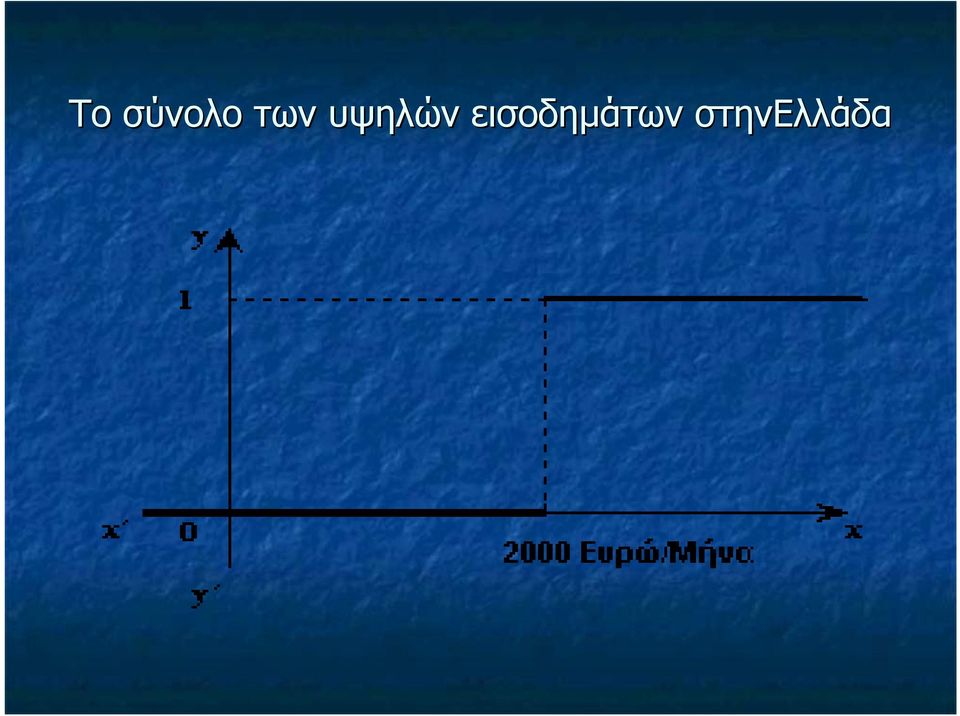
6 Το σύνολο των υψηλών εισοδηµάτων στηνελλάδα

7 Ορισµός του ασαφούς συνόλου Έστω Χ ένα κλασσικό σύνολο αναφοράς.κάθε συνάρτηση: Α: Χ [, ] λέγεται ασαφές υποσύνολο του Χ. Εάν x X,, τότε η τιµή Α(x) λέγεται τιµή συµµετοχής του x (membershp value) ) και εκφράζει τον «βαθµό» που το x «ανήκει» στο ασαφές σύνολο ή αλλιώς το βαθµό αλήθειας της πρότασης.

8 Η έννοια του ασαφούς αριθµού έχει µεγάλη σηµασία στο να παραστήσουµε και να διαχειριστούµε τις γλωσσικές µεταβλητές (lngustc varables) Αυτή η λέξη είναι µια γλωσσική µεταβλητή και βασιζόµενοι µε κάποιο συντακτικό γραµµατικό κανόνα µπορούµε να δώσουµε σε αυτή κάποιες γλωσσικές τιµές (lngustc terms) και έστω ότι οι τιµές που δίνουµε είναι νεαρής ηλικίας, µέσης ηλικίας, µεγάλης ηλικία.

9 Παράδειγµα µιας γλωσσικής µεταβλητής δίνεται η «ηλικία«ηλικία». A (x) Νεαρής ηλικίας : Α Μέσης ηλικίας : Α 2 Μεγάλης ηλικίας : Α x ( Ηλικία σε έτη)

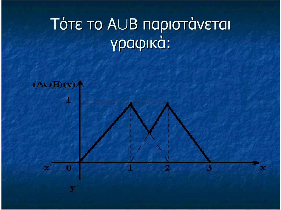
10 Πράξεις Ασαφών Συνόλων Ένωση δύο ασαφών συνόλων Έστω Χ ένα σύνολο αναφοράς και F(Χ) το σύνολο των ασαφών υποσυνόλων του Χ, δηλαδή F(Χ)={Α όπου Α:X [,] }. Αν Α F(Χ), Β F(Χ), τότε το ασαφές σύνολο Α Β Α ορίζεται ως εξής: Α Β F(Χ) µε (Α Β)( Β)(x)= )=max {A(x), B(x)},για κάθε x X. Η ένωση δύο ασαφών συνόλων είναι µία εσωτερική πράξη,, δηλαδή µία απεικόνιση: : F(X) F(X) F(X), έτσι ώστε (Α, Β) Α Β.

11 Τότε το Α Β Α Β παριστάνεται γραφικά:

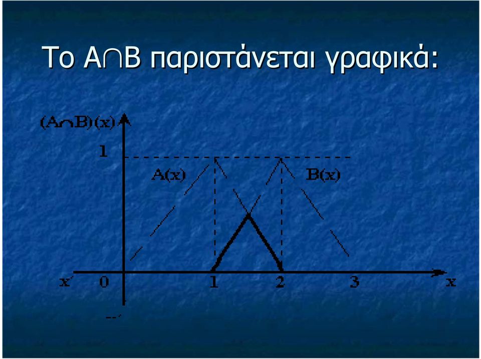
12 Τοµή δύο ασαφών συνόλων Έστω Χ ένα σύνολο αναφοράς και F(Χ) το σύνολο των ασαφών υποσυνόλων του Χ, δηλαδή F(Χ)={Α όπου Α:X [,] }. Αν Α F(Χ), Β F(Χ), τότε το ασαφές σύνολο Α Β Β ορίζεται ως εξής: Α Β F(Χ) µε (Α Β)( Β)(x) ) = mn n {A(x), B(x)},για κάθε x X. Η τοµή δύο ασαφών συνόλων είναι µία εσωτερική πράξη,, δηλαδή µία απεικόνιση: : : F(X) F(X) F(X), έτσι ώστε (Α, Β) Α Β

13 Το Α Β Α Β παριστάνεται γραφικά:

14 Η αρχή της αντίφασης στα ασαφή σύνολα Στα ασαφή σύνολα δεν ισχύει η αρχή της αντίφασης (Α ΑC= ΑC= ) και για να το δείξουµε αυτό αρκεί να δείξουµε ότι υπάρχει ένα τουλάχιστον x X που ικανοποιεί την σχέση: mn[a(x), ),-A(x)] Η σχέση ικανοποιείται για κάθε τιµή A(x) (,) (,) και µόνο για A(x)= ή A(x)= δεν ικανοποιείται.

15 Η αρχή της αντίφασης στα ασαφή σύνολα Γραφική παράσταση του (Α Α c )(x): Γραφική παράσταση των Α(x) και Α c (x):

16 Η αρχή του αποκλειοµενου τρίτου στα ασαφή σύνολα Γραφική παράσταση των Α(x) και Α C (x): Γραφική παράσταση του (Α Α C )(x): ): (A A C) (x) x 2 x y

17

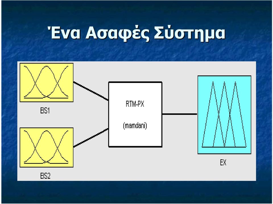
18 Ασαφή Συστήµατα Θα περιγράψουµε ένα ασαφές σύστηµα µε δύο εισόδους (EIS, EIS2) και µια έξοδο (EX). Η ίδια τεχνική µπορεί να επεκταθεί σε προβλήµατα µε περισσότερες εισόδους και εξόδους. Επίσης µπορεί να εφαρµοσθεί και στη περίπτωση που το πρόβληµα έχει µια µόνο είσοδο και µια έξοδο.

19 Ένα Ασαφές Σύστηµα

20 Η διάζευξη Η p q συµβολίζει την διάζευξη δύο προτάσεων µε τιµές αλήθειας: p q p q

21 Η σύζευξη Η p q συµβολίζει την σύζευξη δύο προτάσεων µε τιµές αλήθειας: p q p q

22 Η άρνηση Με p συµβολίζουµε την άρνηση της πρότασης p µε τιµές αλήθειας: p ~p

23 Aσαφής συνεπαγωγή Η διαδικασία της ασαφούς συνεπαγωγής πραγµατοποιείται παράλληλα για όλους τους κανόνες και το αποτέλεσµα για κάθε κανόνα είναι ένα ασαφές σύνολο. Στο σχήµα που ακολουθεί βλέπουµε το αποτέλεσµα µε εφαρµογή της ασαφούς συνεπαγωγής Mamdan, (εννοείται ότι στη θέση της ασαφούς συνεπαγωγής Mamdan µπορεί να χρησιµοποιηθεί κάποια άλλη ασαφής συνεπαγωγή).

24 Η συνεπαγωγή Έστω p, q δύο προτάσεις. Με p q εννοούµε ότι η p συνεπάγεται της q. Ορίζουµε την p q = p q Αυτό σηµαίνει ότι για να βρούµε τον πίνακα αλήθειας του p q αρκεί να βρούµε τον πίνακα αλήθειας της p q:

25 p q ~p ~p q

26 Yπολογισµός της Εξόδου Ασαφούς Συστήµατος αριθµητικές είσοδοι ασαφοποίηση των αριθµητικών εισόδων εφαρµογή ασαφών τελεστών ασαφής συνεπαγωγή συνάθροιση των εξόδων άρση της ασάφειας αριθµητικές έξοδοι

27 Ασαφή Συστήµατα στο MATLAB

28 An optmzaton method for the selecton of the approprate fuzzy mplcaton B. K. PAPADOPOYLOS, G. TRASANIDIS, A. G. HATZIMICHAILIDIS In ths paper we ntroduce a method whch gve us the possblty to choce the most sutable fuzzy mplcaton n nference system s applcaton. We also ntroduce a smlarty measure whch we call degree of sameness two fuzzy mplcatons. Ths smlarty measure gves us the degree of sameness among two fuzzy mplcatons n an nference system s applcaton.

29 ΑΣΑΦΗΣ ΓΡΑΜΜΙΚΗ ΠΑΛΙΝ ΡΟΜΗΣΗ Sample Output Inputs 2.. m y y 2.. y m x, x 2,..., x n 2, x 22,...,x n2 x 2 x m.. m, x 2m,...,x nm

30 Ασαφής γραµµική παλινδρόµηση Αν τη θέση των προσδιοριστέων πραγµατικών αριθµών α, α2,, αν, c πάρουν ασαφείς αριθµοί Α,Α2,,Αν,Α τότε προκύπτει ένα µοντέλο ασαφούς γραµµικής παλινδρόµησης της µορφής: Α x +Α 2 x 2 + +Α ν x ν +Α =Y

31 y c c 2 r x Aν ν οι ασαφείς αριθµοί Α,Α2,,Αν,Α είναι τριγωνικοί τότε το αποτέλεσµα είναι ο ασαφής τριγωνικός αριθµός Y(r-c, r, r+c2), όπου c,,c2.

32 m n J = mn mc + c x j j= = m n J = mn mc + c j= = n n y r + r x ( h) c + c x j j j = = n n y r + r x + ( h) c + c x j j j = = c, =,2,, n x j

33 Orgnal paper Soft Computng 8 (24) Ó Sprnger-Verlag 23 DOI.7/s y Smlartes and dstances n fuzzy regresson modelng B. K. Papadopoulos, M. A. Srp 556 Abstract We study the set of the solutons of a fuzzy regresson model as a metrc space. For each metrc, we defne a smlarty rato n order to compare the spaces of solutons of a fuzzy regresson model. We prove that the smlarty ratos, that can be extracted from these dfferent metrcs, are all the same as n [4]. As an applcaton, we use the smlarty rato to produce fuzzy classfcaton of models. A numercal example, nvolvng economc data, s gven. Keywords Fuzzy regresson analyss, Metrc spaces, Smlartes, Fuzzy classfcaton Introducton In classcal statstcal regresson, the relatonshp between the nputs and the output s sharp. Any devaton between the estmated and the observed values s attrbuted to varous reasons and reflected n the dsturbance term. In contrast to the statstcal regresson, the fuzzy one has no dsturbance term and the dfferences between the observed and the computed values are reflected n the parameter fuzzness. The more the wdth of a parameter s, the lees we know about the contrbuton of the varable n the model, but stll we have an ncomplete knowledge of t. For ths reason fuzzy regresson analyss offers an effcent tool for analysng complex systems, such as economc systems, socal systems, envronmental systems, where the vagueness of human subjectve judgement s nfluental. Let for a fuzzy lnear regresson model, we have dfferent sets of data that come from dfferent stuatons and we want to determne whether the derved models are nherently dfferent or not. Usng approprate metrcs, we prove that the set of solutons of a fuzzy lnear regresson model consttute a metrc space. Afterwards, a smlarty Publshed onlne: 23 September 23 B. K. Papadopoulos (&) Democrtus Unversty of Thrace, Department of Cvl Engneerng, 67 Xanth, Greece E-mal: papadob@cvl.duth.gr M. A. Srp Unversty of Macedona, Department of Appled Informatcs, Alex. Mchalds str. 4, Thessalonk, Greece The research reported n ths paper was carred out n the framework of MathInd Project rato s used as a test of convergence, ether between the fuzzy models or wth respect to ther fuzzness. As measure of closeness, the smlarty rato gves a bnary fuzzy relaton n the set of the models, whch can be used for dfferent knds of fuzzy classfcatons. 2 Fuzzy lnear regresson for fuzzy output data A fuzzy lnear regresson model has the followng form: Y ¼ A þ A X þ A 2 X 2 þþa n X n ðþ where A ; ¼ ;...; n are symmetrcal fuzzy numbers []. Accordng to Tanaka et al. [5, 6], we assume that nput data consttute a vector of nonfuzzy numbers and output data s a fuzzy number, beng the devatons caused by the ambguty of the system structure. For n ndependent varables and m samples, we arrange our data as follows: Then we have the followng system: Y ¼ XA ð2þ where y x x 2 x n y 2 x 2 x 22 x n2 Y ¼ ; X ¼ ; y m x m x 2m x nm 2 3 A A A ¼ A n wth A and Y vectors of fuzzy numbers. The components of A are symmetrcal trangular fuzzy numbers wth membershp functons: l A ða Þ¼L a r c ; c > ; r ; c are the centre and spread, respectvely ð3þ where L ðxþ ¼maxð; jxjþ and s such that L ðxþ ¼ L ð xþ, L ðþ ¼, L ðxþ strctly decreasng n ½; Þ. When the parameters of the fuzzy lnear regresson model are symmetrcal trangular fuzzy numbers, usng the extenson prncple, the outputs Y j of the system (2) are also symmetrcal trangular fuzzy numbers, wth membershp functons [6]:

34 P y j r þ n r x j ¼ l Yj ðy j Þ¼L B c þ Pn A c jx j j ¼ ð4þ The problem of fndng the parameters of the lnear system (2), s converted to a lnear programmng problem n the followng way: (a) Intally we consder the model: Y j ¼ A þ A x j þ A 2 x 2j þþa n x nj ; j ¼ ; 2;...; m where A ¼ðr ; c Þ L ¼ðr c ; r ; r þ c Þ T are symmetrcal trangular fuzzy numbers. (b) We determne thedegree h to whch we wsh the data ðx j ; x 2j ;...; x nj Þ; y j to be ncluded n the nferred number Y j, that s l Yj ðy j Þh for j ¼ ; 2;...; m, and hence (4) takes the form: P y j r þ n r x j ¼ l Yj ðy j Þ¼L B c þ Pn A c x j h ð5þ ¼ (c) So we take the followng objectve functon:! J ¼ mn Xm c þ Xn c x j j¼ ¼ ð6þ In other words from (5) and (6), we get the followng Lnear Programmng (LP) problem:! J ¼ mn Xm c þ Xm X n c x j ð7þ j¼ y j r þ Xn ¼ y j r þ Xn ¼ j¼ ¼ r x j ð hþ r x j þð hþ c þ Xn ¼ c þ Xn ¼ c x j c x j!! ð8þ ð9þ c ; ¼ ; ;...; n ðþ It s known [6] that, for the data n Table, there s an optmal soluton A h ¼ðr h ; ch Þ L ; ¼ ;...; n; h < : The optmal soluton A h ¼ðr h ; c h Þ L ; ¼ ;...; n for any other level h 6¼ h can be obtaned from the optmal h level soluton n the followng way: Table. Sample Output Inputs y x ; x 2 ;...; x n 2 y 2 x 2 ; x 22 ;...; x n m y m x m ; x 2m ;...; x nm A h ¼ r h ; h h ch L ðþ 3 The metrc space of fuzzy lnear regresson models It s known that trangular fuzzy numbers A ¼ða ; a 2 ; a 3 Þ T, wth a a 2 a 3, have a membershp functon, whch has n general the followng form: 8 for x a >< x a l A ðxþ ¼ a 2 a for a < x a 2 a 3 x a 3 a 2 for a 2 < x a >: 3 for a 3 < x ð2þ Gven two trangular fuzzy numbers A ¼ða ; a 2; a 3 Þ T and B ¼ðb ; b 2 ; b 3 Þ T, then a proposed dstance s: DðA; BÞ ¼ ½ 2 max ðj a b j; ja 3 b 3 jþ ja 2 b 2 jþš ð3þ If we have two symmetrcal trangular fuzzy numbers, A ¼ðr ; c Þ L ¼ ðr c ; r ; r þ c Þ T and B ¼ðr 2 ; c 2 Þ L ¼ ðr 2 c 2 ; r 2 ; r 2 þ c 2 Þ T the above dstance can be calculated by the followng formula: DðA; BÞ ¼ 2 ½ max ðj r c r 2 þ c 2 j; jr þ c r 2 c 2 jþ jr r 2 jþš ð4þ Consderng agan the data of Table and supposng that the optmal soluton of the LP problem has been calculated for level h, then we have the fuzzy regresson model: M h : Yj h ¼ A h þ Ah x j þ A h 2 x 2j þþa h n x nj; j ¼ ;...; m ð5þ where, A h ¼ r h; ch ; ¼ ;...; n have been calculated from the LP problem. Let M ¼ M h : h 2½; Þ be the set of all such models for all dfferent levels. Ths leads us to the followng defnton: Defnton 3.. The dstance D between two models M h and M h 2 of M s defned as follows: DðM h ; M h 2 Þ¼ Xn ¼! =2 D 2 A h ; A h 2 ð6þ So D s a metrc n M and consequently we have the metrc space (M, D) by the followng proposton. Proposton 3.2. The dstance D between two models M h and M h 2 of M, s of the followng form: D M h ; M h jh 2 h 2 j ¼ 2ð h Þð h 2 Þ q ffffffffffffffffffffffffffffffffffffffffffffffffffffffffffffffffffffffffffffffffffffffffffffffffffffff ðc Þ2 þðc Þ2 þþðc n Þ2 Proof. Let A h ¼ r h ; c h ; ¼ ; ; 2;...; n and L A h 2 r h 2 ; c h 2 ; ¼ ; ; 2;...; n. By the relaton () t L ð7þ 557

35 558 follows that r h ¼ r h 2 ¼ r, ch h c and c h 2 ¼ h 2 c ; ¼ ; ;...; n. So, D 2 M h ; M h X n 2 ¼ 2 max ch þ c h 2 ; c h c h 2 2 and thus, ¼ ¼ Xn ¼ X n ¼ 4 ¼ 4 ¼ 2 4 ch c h 2 2 ¼ c h c h 2 h h 2 ð h Þð h 2 Þ 2X n ¼ c 2 DðM h ; M h 2 jh h 2 j Þ¼ 2ð h Þð h 2 Þ qffffffffffffffffffffffffffffffffffffffffffffffffffffffffffffffffffffffffffffffffffffffffffffffffffffff ðc Þ2 þðc Þ2 þþðc n Þ2 Proposton 3.3. If h h 2 and h h 3, then D M h ; M h 2 D M h ; M h 3 ff h2 h 3. Proof. Settng D M h ; M h ðh 2 2 h Þ ¼ 2ð h Þð h 2 Þ qffffffffffffffffffffffffffffffffffffffffffffffffffffffffffffffffffffffffffffffffffffffffffffffffffffff ðc Þ2 þðc Þ2 þþðc n Þ2 ; D M h ; M h ðh 3 3 h Þ ¼ 2ð h Þð h 3 Þ qffffffffffffffffffffffffffffffffffffffffffffffffffffffffffffffffffffffffffffffffffffffffffffffffffffff ðc Þ2 þðc Þ2 þþðc n Þ2 we have the followng relatons: D M h ; M h 2 D M h ; M h ðh 3 2 h Þ, h 2 ð h 3 h Þ, h 2 h 3 : h 3 Corollary 3.4. D M ; M h D M ; M h 2 ff h h 2. Proposton 3.5. The metrc space ðm; DÞ s stable n the followng sense: 8 h 2½; Þ; 8 e > ; 9 d > ; D M h ; M hþd < e Proof. Let h 2½; Þ be gven and let e > be arbtrary. Then we have: D M h ; M hþd d < e, 2ð hþð h dþ qffffffffffffffffffffffffffffffffffffffffffffffffffffffffffffffffffffffffffffffffffffffffffffffffffff 2þ c h c h 2þþ c h 2 n < e ð8þ If we set A ¼ q ffffffffffffffffffffffffffffffffffffffffffffffffffffffffffffffffffffffffffffffffffffffffffffffffffff 2þ c h c h 2þþ 2ð hþ c h 2 n the relaton (8) s equvalent wth the relaton: d h d A < e, d < e eh A þ e : In the followng Proposton, we observe that the metrc space ðm; DÞ behaves equally well as the metrc space ½; Þ equpped wth the usual metrc. Proposton 3.6. The metrc spaces ðm; DÞ and ½; Þ are homeomorphc. Proof. We consder the functon f : ½; Þ!M; f ðhþ ¼M h ; for each h 2½; Þ: We prove that f s contnuous. Let an h 2½; Þ, and consder and a sequence fh n ; n 2 Ng ½; Þ, such that lm h n ¼ h. We prove that lm M h n ¼ M h. It holds that D M h n ; M h jh n h j ¼ A ; h n where q ffffffffffffffffffffffffffffffffffffffffffffffffffffffffffffffffffffffffffffffffffffffffffffffffffff 2þ A ¼ c h c h 2þþ 2ð h Þ c h 2 n and obvously, lm D M h n ; M h jh n h j ¼ lm A ¼ : h n Conversely, f lm M h n ¼ M h, then lm h n h h n ¼, whch mples that lm h n ¼ h. Let us now use the symbol M d ¼ M h d : h 2½; Þ to emphasze the fact that all M h d are extracted from a set of data, lke those ones of Table. Then the next Theorem follows mmedately: Theorem 3.7. M d s homeomorphc to M d for each par of data d and d. Let now : M d! M d be the functon defned by M h d ¼ M h d, for each Mh d 2 Md. Then the followng Theorem holds: Theorem 3.8. The mappng : M d! M d s a smltude wth rato j where P n c 2 d ¼ j ¼ B P n 2 A ð9þ d ¼ c that s D M h d ; Mh 2 d ¼ j; for each h ; h 2 2½; Þ D M h d ; Mh 2 d

36 Proof. From relaton (7) we can mmedately extract that: vffffffffffffffffffffffffffffffffffffffffffffffffffffffffffffffffffffffffffffffffffffffffffffffffffffffff D M h d ; Mh 2 d ðc Þ 2 d ¼ þ ð c Þ 2 d þþ u 2 t c n d D M h d ; Mh 2 ðc d Þ 2 d þ ð c Þ 2 d þþ 2 ¼ j c n d Remark 3.9. If j ¼, then the mappng of the prevous Theorem s an sometry, that s D M h d ; Mh 2 d ¼ D M h d ; Mh 2 for each h d ; h 2 2½; Þ. Let us now consder the spaces M d and M d wth respect to the smlarty. For ths purpose we gve the followng defnton: Defnton 3.. From the gven sets of data d and d we suppose the spaces M d and M d of fuzzy lnear regresson models have the same varables. We defne as smlarty rato of these two models the followng number: kðd; d Þ¼mnfj; =jg Obvously, < k. ð2þ 4 Smlarty rato based on fuzzness of the regresson model It s known that gven a fuzzy number A n X ¼½a; bš, a measure of fuzzness of A s gven by the formula: f ðaþ ¼ Z b a ð j2l A ðxþ jþdx ¼ b a Z b a ðj2l A ðxþ jþdx : If A ¼ðr c; r; r þ cþ T, then l A ðxþ ¼ jr xj c for r c x r þ c otherwse hence f ðaþ ¼2c c 2c2 c 2 ¼ c : Defnton 4.. If A h ¼ðr h ; c h Þ L ; ¼ ;...; n; A h 2 ¼ðr h 2 ; c h 2 Þ L ; ¼ ;...; n are the solutons of the PL problem, we defne a dstance D f between A h and A h 2 : D f A h ; A h 2 ¼ f A h f A h 2 ¼ c h c h 2 ð2þ Defnton 4.2. The dstance D f between two models M d and M d of M s defned as follows: ðd f Þ M h ; M h X n 2 ¼ ¼ h! =2 2 ðd f Þ A h ; A h 2 ð22þ Proposton 4.3. The dstance D f between two models d and M d of M has the followng form: D f M h ; M h 2 2 qffffffffffffffffffffffffffffffffffffffffffffffffffffffffffffffffffffffffffffffffffffffffffffffff jh h 2 j ¼ ðc Þ 2 þðc Þ 2 þþ c ð h Þð h 2 Þ 2 n ð23þ Proof. Obvous Remark 4.4. Snce D M h ; M h 2 ¼ 2 D f M h ; M h 2 2, the metrcs D and D f are topologcally equvalent. So the Propostons 3.3, 3.5 and 3.6 also holds for D f. Also the theorem 3.8 holds and t can be extracted the same smlarty rato, snce D f M h d ;Mh 2 d ¼k f ðd;d Þ D f M h d ;Mh 2 d 8 P n =2 c 2 P n 9 =2 c d ¼ 2 >< d ¼mn B C ¼ P n c 2 A ; B P n A ¼kðd;d Þ >: c d >; ¼ for each h ; h 2 2½; Þ. Remark 4.5. In [4] we have ntroduced the same smlarty rato based on Hammng dstance. Remark 4.6. The smlarty rato express not only the metrc dstance between two fuzzy models but also expresses the dfference of fuzzness of the models. 5 An applcaton of smlarty rato n fuzzy classfcaton Suppose now we have a set Y of m objects and we wsh ther fuzzy classfcaton. We have frst to assgn values at the elements of ther membershp matrx. In the case that the objects are descrbed by n numerc varables we can substtute resemblance coeffcents [2] between each par of objects n place of ther values. Ths method s based on the statstcal aspects of the data. Here, nstead of resemblance coeffcents, we wll use the smlarty ratos among the objects as entres n the membershp matrx. Then, the fuzzy classfcatons, based on the fuzzy characterstcs of the objects, wll be possble. Let Y ¼ ^Y ; ^Y 2 ;...; ^Y n be the set, whose objects are the fuzzy outputs estmated from the dfferent sets of data ðd ; d 2 ;...; d n Þ va fuzzy lnear regresson models. Usng the relatons (9) and (2) for each par ^Y ; ^Y j 2 Y Y, we can compute a smlarty rato k j. The smlarty rato gves a bnary fuzzy relaton R on Y 2 n the followng way: l R : Y Y!ð; Š wth l R ^Y ; ^Y j ¼ kj ð24þ where k j ¼ mn j j ; =j j ; and ¼ 2 d 559

37 56 vffffffffffffffffffffffffffffffffffffffffffffffffffffffffffffffffffffffffffffffffffffffffffffffffffffffff ðc Þ 2 d j j ¼ þðc Þ 2 d þþ c 2 u n d t ðc Þ 2 d j þðc Þ 2 d j þþ c n 2 d j ð25þ We can say, that the defned fuzzy relaton represents the concept very near. Also, k ¼ and snce j j ¼ =j j, k j ¼ mn j j ; =j j ¼ mn =jj ; j j ¼ kj the matrx has the followng form 2 3 k 2 k n k 2 k n2 R ¼ k n k n2 ð26þ It s known [3], that a fuzzy relaton R s: (a) relexve ff l R ^Y; ^Y ¼, for all ^Y 2 Y, (b) symmetrc ff l R ^Y ; ^Y j ¼ lr ^Y j ; ^Y and (c) transtve (or max-mn transtve) ff l R ^Y ; ^Y j max mn l ^Y R ; ^Y k ; lr ^Y k ; ^Y j s satsfed k¼;...;m for each par ^Y ; ^Y j 2 Y 2. Obvously, the defned fuzzy relaton R s always reflexve and symmetrc. By consderng the basc propertes (reflexvty, symmetry and transtvty), we can dstngush 2 dfferent types of bnary fuzzy relatons and execute 4 dfferent types of fuzzy classfcaton.. A fuzzy bnary relaton that s reflexve, symmetrc and transtve s known as a fuzzy equvalence relaton or smlarty relaton. If the relaton R s a smlarty relaton, we can execute two types of classfcaton n Y [3]. Frstly, for each ^Y 2 Y we can fnd a smlarty class. Ths concdes wth the fuzzy set n whch the membershp degree of any partcular element represents the smlarty of that element to the element ^Y. In our case, ths wll be the fuzzy set S ^Y ¼ ^Y j ; k j ; j ¼ ; 2;...; n ð27þ Secondly, we can group the objects of Y nto crsp sets whose members are near to each other to some specfed degree. Denote K R the level set, whch s the set of all membershp values appearng n the matrx,.e. K R ¼ k j ; ; j ¼ ;...; n ð; Š ð28þ Then for any a 2 K R, we can take an a-cut a R of R, whch s a crsp equvalence relaton that represents the presence of closeness between the objects to the degree a. Ths crsp equvalence relaton s gven by a R ¼ ^Y ; ^Y j =kj a ð29þ Each of these equvalence relatons forms a partton p a ð RÞ ¼ p a ; pa 2 ;...; pa k ð3þ and t holds that ^Y 2 Y ^Y j 2 Y ^Y ; ^Y j 2 p a l, k j a ð3þ the set PðRÞ ¼fpð a RÞ=a 2 K R g of all parttons of Y can be convenently dagrammed by a partton tree. 2. A fuzzy bnary relaton that s reflexve and symmetrc s called a fuzzy compatblty relaton. When our relaton s a fuzzy compatblty relaton, we can execute two types of classfcaton n Y. Frstly, gven a compatblty relaton, for each a 2 K R we can determne ts maxmal a-compatble. Amaxmal a-compatble s a subset a C of Y, whch s defned by the followng propertes: 8^Y 2 a C 8^Y j 2 a C kj a ð32þ and a C 6 a C j ; 6¼ j ð33þ The famly a CðRÞ ¼ C a; Ca 2 ;...; Ca k consstng of all maxmal a-compatbles, nduced by R on Y, s called complete a-cover of Y wth respect to R. Ths set, for some values of a, forms parttons of Y. The set CðRÞ ¼f a CðRÞ=a 2 K R g of all complete a-covers of Y can be convenently dagrammed by a tree. Secondly, although the relaton s not transtve, we wsh for every a 2 K R to take a partton of Y, and determne the transtve closure R T. To ths end, we use the followng algorthm [3]: R T ¼ R R R ðn tmesþ ð34þ beng the max-mn composton. So, for the elements k j of the membershp matrx of R T, t holds that k j ¼ k j ; k j ¼ max k j; max mn k k ; k kj ; k ¼ k¼;...;n ð35þ We can fnd the set PðR T Þ¼fnp ð a R T Þ=a 2 K R goof all parttons of Y, whose blocks p a T ; p a T 2 ;...; p a T k are defned by the relaton ^Y 2 Y ^Y j 2 Y ^Y ; ^Y j 2 p a l, k j a ð36þ Thus, a fuzzy classfcaton, based on fuzzy regressons, comprses the followng steps.. Arrange the sets of data n Tables (as Table ). 2. Settng h ¼, for each Table fnd the fuzzy coeffcents usng relatons (7) (). 3. Compute the smlarty ratos usng the relatons (25). 4. Formulate the membershp matrx R gven by (26). 5. Determne the transtve closure R T usng (34) or the relatons (35). 6. If the relaton 2s proved to be a smlarty relaton go to 7, otherwse go to Fnd the smlarty classes as n (27) or the set PðRÞ ¼fpð a RÞ=a 2 K R g of all parttons of Y, usng the relatons (28), (3) and (3). Stop. 8. Fnd CðRÞ ¼f a CðRÞ=a 2 K R g of all complete a-covers of Y, usng the relaton (28), (32) and (33). 9. Use R T determned n step 5, to fnd the set PðRÞ ¼fpð a RÞ=a 2 K R g of all parttons of Y, usng relatons (28), (36).. End.

38 Table 2. r c r c r 2 c 2 Span Portugal France Germany Table 3. Span Portugal France Germany Fg Span Portugal France Germany Fg.. A numercal example As an applcaton, we wll use the well-known consumpton functon C t ¼ a þ a Y t þ a 2 C t and data from four countres, namely France, Germany, Portugal and Span, concernng the perod The orgnal data are retreved from the 995 s Internatonal Fnancal Statstcs Yearbook, and transformed at fxed 99 s ECU prce, so the fuzzy lnear regresson models we computed assume the form: C t IPD CR ¼ A þ A GNP t IPD CR þ A 2 C t IPD CR where A ¼ ðr ; c Þ L are the symmetrcal trangular fuzzy coeffcents, C = prvate Consumpton n current prces, GNP = Gross Natonal Income n current prces, IPD = Implct Prce Deflator (99 = ), CR = 99 Converson Rate ( ECU =...) Solvng four PL problems, one for each country, we extract the followng results: Usng (25) we extract the followng smlartes ratos: Then S P F G 2 3 S :429 :769 :3226 R ¼ P F G :429 :33 : :769 :33 :495 5 :3226 :38 :495 Usng the algorthm (34) or (35), we fnd S P F G S 2 3 R T ¼ P :429 :769 :495 :429 :429 : F :769 :429 : ¼ R G :495 :429 :495 Snce R T 6¼ R we know that the relatonshp s a fuzzy compatblty relaton. The level set s K R ¼ f; :769; ; 3226; :33; :38g. The set of all complete a-covers s depcted by the followng tree: The level set for R T s K RT ¼ f; :769; :495; :429g and then the set of all parttons s depcted from the followng tree: References. Bardossy A, Ducksden L (995) Fuzzy Rule-Based Modellng wth Applcatons to Geophyscal, Bologcal and Engneerng Systems. CRC Press, Boca Raton 2. Huhua X, Henry JJ (99) The Use of Fuzzy-Sets Mathematcs for Analyss of Pavement Skd Resstance. In: Meyer WE, Rechert J (eds) Surface Characterstcs of Roadways: Internatonal Research and Technologes, ASTM STP 3, Amercan Socety for Testng and Materals, Phladelpha, pp Klr GJ, Yuan B (995) Fuzzy Sets and Fuzzy Logc: Theory and Applcatons. Prentce-Hall, Englewood Clffs, New Jersey 4. Papadopoulos BK, Srp MA (999) Smlartes n Fuzzy Regresson Models. Journal of Optmzaton Theory and Applcatons 2(2): Tanaka H, Uejma S, Asa K (982) Lnear Fuzzy Regresson Analyss wth Fuzzy Models. IEEE Tran. Syst. Man Cybernet SMC (2): Tanaka H (987) Fuzzy Data Analyss by Possblstc Lnear Models. Fuzzy Sets and Systems (24): Terano T, Asa K, Sugeno M (992) Fuzzy Systems Theory and ts Applcatons. Academc Press, Harcount Brace Jovanovch Publshers, San Dego, Calforna

39 AN OPTIMIZATION METHOD FOR THE SELECTION OF THE APPROPRIATE FUZZY IMPLICATION B. K. Papadopoulos, G. Trasandes, A. G. Hatzmchalds Department of Cvl Engneerng Democrtus Unversty of Thrace GR-67 Xanth, Greece hatz February 25 Abstract In ths paper we ntroduce a method whch gves us the possblty to choose the most sutable fuzzy mplcaton, n an nference system s applcaton. We also ntroduce a smlarty measure, whch we call degree of sameness of two fuzzy mplcatons, n an nference system s applcaton. Keywords: metrc dstance, smlarty, fuzzy mplcaton Introducton and Prelmnares. Fuzzy Implcatons, Notatons and Basc Defntons All the defntons and notatons on fuzzy mplcatons, that we are gong to use n ths paper, can be found n [3], [4], [5]. [7] and [8]. Defnton A fuzzy mplcaton, σ, s a functon of the form: σ : [, ] [, ] [, ], whch defnes (for any possble truth values a, b of gven fuzzy propostons p, q respectvely) the truth value σ(a, b) of the condtonal proposton f p then q.

40 The functon σ should be an extenson of the classcal mplcaton from the doman {, } to the doman [, ], of truth values n fuzzy logc. Defnton 2 The mplcaton operator of classcal logc s a mappng: m : {, } {, } {, }, whch satsfes the boundary condtons: m(, ) = m(, ) = m(, ) and m(, ) =. These condtons are the least ones that we can demand from an mplcaton operator. In other words, fuzzy mplcatons collapse to the classcal mplcaton, when the truth values are restrcted between and : σ(, ) = σ(, ) = σ(, ) = and σ(, ) = In fact, there are many dfferent fuzzy mplcatons and the most of them ft nto one of the followng three general cases: () the S mplcatons: σ S (a, b) = n(a) b, for all a, b [, ]; () the R mplcatons: σ R (a, b) = sup{x [, ]/a x b}, for all a, b [, ] and () the QL mplcatons: σ QL (a, b) = n(a) (a b), for all a, b [, ], where s a t norm, s a t conorm, n s a strong negaton and the trple <,, n > must satsfy the De Morgan laws..2 Metrc Dstances, Notatons and Basc Defntons Defnton 3 A metrc dstance d, n a set A, s a real functon d : A A R, whch satsfes the followng condtons: () d(x, y) = x = y; () d(x, y) = d(y, x) (symmetrc) and () d(x, z) + d(z, y) d(x, y) (trangle nequalty), where x, y, z A. Defnton 4 A par (X, Y ) of a set X and a metrc d, on X, s called metrc space. 2

41 Some common metrcs, whch are used to descrbe the dstance between fuzzy sets, are the followng (see also [2], [6]): () the Eucldean dstance: d E (µ, ν) = Σ n = (µ(x ) ν(x )) 2 and () the Hammng dstance: d H (µ, ν) = Σ n = µ(x ) ν(x ), where we consder X = {x,..., x n } to be a fnte unverse set and for any two fuzzy subsets A and B the membershp functons are µ and ν respectvely. 2 A Method for measurng Dstances between Fuzzy Implcatons One of the most common problems n buldng an nference system s the choce of a sutable fuzzy mplcaton. Here we propose a specfc method, whch s based on generalsed modus ponens, and whch solves ths problem. It s mportant that ths method s based on the choce of a sutable fuzzy mplcaton. In partcular, we consder measurements of x as an nput, wth correspondng degrees of truth B(y ), and the correspondng measurements of y as an output, wth degrees of truth B(y ). Let now σ (κ, λ), σ 2 (κ, λ) be two fuzzy mplcatons, where κ, λ [, ]. We would lke to choose the most sutable one, and we propose an algorthm for ths, whch follows after the followng two defntons, whch are qute mportant: Defnton 5 Let A = a /x + a 2 /x a n /x n and B = b /y + b 2 /y b n /y n be two fuzzy subsets of the sets X = {x, x 2,..., x n } and Y = {y, y 2,..., y n } respectvely. Let also σ be a fuzzy mplcaton. We defne the matrx of the fuzzy mplcaton σ as follows: σ(a, b ) σ(a, b 2 )... σ(a, b n ) σ(a 2, b ) σ(a 2, b 2 )... σ(a 2, b n ) σ(a(x ), B(y j )) = , σ(a n, b ) σ(a n, b 2 )... σ(a n, b n ) where, j =,..., n. Defnton 6 Let be an approprate t norm, such that the low of modus ponens holds. Then, the n matrx of [B σ (y ), B σ (y 2 ),..., B σ (y n )] s equal 3

42 to: [A(x ), A(x 2 ),..., A(x n )] usng max matrces. σ(a, b ) σ(a, b 2 )... σ(a, b n ) σ(a 2, b ) σ(a 2, b 2 )... σ(a 2, b n ) σ(a n, b ) σ(a n, b 2 )... σ(a n, b n ) So, we would lke to calculate B σ (y ),..., B σ (y n ) and B σ2 (y ),..., B σ2 (y n ), where σ, σ 2 are fuzzy mplcatons. Between σ and σ 2 we choose as the most sutable fuzzy mplcaton ths one, whose dstance of B σk (y ),..., B σk (y n ), k =, 2, from the values of [B(y ), B(y 2 ),..., B(y n )], of the output, s the smallest one. So, now we have the machnery to ntroduce our algorthm, whch we dvde nto four steps: () We calculate the n n matrx σ (A(x ), B(y ))., () We then calculate the n n matrx: σ(a, b ) σ(a, b 2 )... σ(a, b n ) σ(a 2, b ) σ(a 2, b 2 )... σ(a 2, b n ) [A(x ), A(x 2 ),..., A(x n )] σ(a n, b ) σ(a n, b 2 )... σ(a n, b n ), usng max matrces, where s a contnuous t norm. () We now calculate the n matrx: B σ (y ),..., B σ (y n ) (v) Last, we calculate the dstance d(b, B σ ), between [B(y ), B(y 2 ),..., B(y n )] and B σ (y ),..., B σ (y n ), usng a metrc dstance between two fuzzy sets. We repeat the steps ()-(v) for the fuzzy mplcaton σ 2, and we calculate the dstance d(b, B σ2 ). Then, we choose as the most sutable fuzzy mplcaton, between σ and σ 2, the one havng the smallest dstance, d. We arrange our data n a tabular form, as follows: x A(x ) y B(y j ) σ(a(x ), B(y j )) B σ (y j ) = max( [A(x ), σ (A(x ), B(y j ))]) x A(x ) y B(y ) a j = σ (A(x ), B(y j )) B σ (y ) = max( [A(x ), a ]) x 2 A(x 2 ) y 2 B(y 2 ) a 2j = σ (A(x 2 ), B(y j )) B σ (y 2 ) = max( [A(x ), a 2 ]) x n A(x n ) y n B(y n ) a nj = σ (A(x n ), B(y j )) B σ (y n ) = max( [A(x ), a n ]) 4

43 We wll now llustrate ths algorthm, by gvng an example. In ths example we compare the two well known fuzzy mplcatons (whch are used n nference systems) namely: () The Mamdan mplcaton: σ M (A(x ), B(y j )) = A(x ) B(y j ) and () the Larsen mplcaton: σ L (A(x ), B(y j )) = A(x ) B(y j ). We remark that these two mplcatons do not collapse wth the classcal mplcaton, when the truth values are restrcted to and to,.e. σ M (, ) = σ L (, ) =. Example Let x be the nput data and let also A =./x +.4/x 2 +.6/x 3 be the fuzzy set wth unverse set X = {x, x 2, x 3 }. Let y j be the output data and B =.2/y +.3/y 2 +.7/y 3 be the fuzzy set wth unverse set Y = {y, y 2, y 3 }. When we obtan the Mamdam mplcaton, σ M (A(x ), B(y j )) = A(x ) B(y j ), we get: σ M (A(x ), B(y j )) = Also, by the matrx multplcaton: [.,.4,.6] usng the mn-max, we get: [.2,.3,.6] ,. Hence, B σm (y ), B σm (y 2 ), B σm (y 3 ) = [.2,.3,.6]. In a smlar way, let us consder the followng fuzzy sets: A =./x +.4/x 2 +.6/x 3, B =.2/y +.3/y 2 +.7/y 3, x X, y Y and the Larsen mplcaton: We obvously get the matrx: σ L (A(x ), B(y j )) = A(x ) B(y ) σ L (A(x ), B(y j )) =

44 () Choosng the algebrac product (a, b) = ab, we get: [.,.4,.6] and usng the max we get: [.72,.8,.252] Hence, B σl (y ), B σl (y 2 ), B σl (y 3 ) = [.72,.8,.252]. () When we use the standard fuzzy ntersecton, we get: [.,.4,.6] and usng the mn-max, we get: [.2,.8,.42] Hence, B σl (y ), B σl (y 2 ), B σl (y 3 ) = [.2,.8,.42]. We can calculate the dstance between two fuzzy mplcatons, usng the Hammng dstance d H (A, B) = Σ n = A(x ) B(x ), as follows: d M H (B, B σm ) = Σ 3 j= B(y j ) B σm (y j ) =., d L H (B, B σ L ) =.768, d L H (B, B σl ) =.48. So, n ths case we propose as the most sutable mplcaton the Mandan one, and the most sutable after the Mandam s the Larsen one, usng mnmax matrces. 3 A Smlarty Measure for Fuzzy Implcatons We wll now ntroduce three measures of smlarty for two fuzzy sets A and B, n a fnte unverse set X. [9] 6

45 M(A, B) = { f A = B = P x X mn(a(x),b(x)) x X max(a(x),b(x)) otherwse L(A, B) = max x X A(x) B(x) { f A = B = S(A, B) = P x X A(x) B(x) x X A(x)+B(x) otherwse When we consder the measure L(A, B), for fuzzy sets A and B n arbtrary unverses, we have to replace max wth sup. Furthermore, we ntroduce the smlarty measure called degree of sameness, by Bandler and Kohout ([],[]): E(A, B) = mn(nf x X σ(a(x), B(x)), nf x X σ(b(x), A(x)) Last, but not least, we defne the smlarty measure whch we call degree of sameness of two fuzzy mplcatons σ and σ 2, as follows: ( Bσ (y j ) S(σ, σ 2 ) = mn B σ2 (y j ), B ) σ2(y j ), B σ (y j ) where s a norm on X and B σ, B σ2 were ntroduced n secton 2, n the 3rd step of our algorthm. Example 2 We consder the followng fuzzy sets: A =./x +.4/x 2 +.6/x 3, B =.2/y +.3/y 2 +.7/y 3, x X, y Y, from the Example, so we get: B σm (y ), B σm (y 2 ), B σm (y 3 ) = [.2,.3,.6] and B σl (y ), B σl (y 2 ), B σl (y 3 ) = [.2,.8,.42] When we choose the norm A(x ) = n = A(x ), the degree of sameness of the above mplcatons s: ( BσM (y j ) S(σ M, σ L ) = mn B σl (y j ), B σ (y ) ( L j). = mn B σm (y j ).72,.72 ) = mn(.527,.654). =.654 When we choose the Eucldean norm A(x ) 2 = ( n = A(x ) 2 ) /2, the degree of sameness of these mplcatons s: ( BσM (y j ) 2 S(σ M, σ L ) = mn, B σ (y L j) 2 B σl (y j ) 2 B σm (y j ) 2 =.67 7 ) (.7 = mn.47,.47 ) = mn(.489, 67).7

46 Conclusons In ths paper we ntroduced an algorthm that calculates the dstance between two fuzzy mplcatons. We also ntroduced a smlarty measure, whch we call degree of sameness, of two fuzzy mplcatons. References [] W. Bandler and L. Kohout Fuzzy Power Sets and Fuzzy Implcaton Operators, Fuzzy Sets and Systems 4 (98), 3-3. [2] P. Damond and P. Kloeden Metrc Spaces of Fuzzy Sets Theory and Applcatons, World Scentfc Publshng Co. Pte. Ltd, Sngapore, 994. [3] D. Dubos, H. Prade Fuzzy Sets and Systems: Theory and Applcatons, Academc Press, New York, 98. [4] D. Dubos, H. Prade Fuzzy Sets n Approxmate Reasonng, part : Inference wth Possblty Dstrbutons, Fuzzy Sets and Systems 4 (99), [5] Fodor, J. C., M. Roubens Fuzzy Preference Modellng and Multcrtera Decson Support, Theory and Decson Lbrary, Kluwer Academc Publshers, Dordrecht, 994. [6] J. Kacprzyk Multstage Fuzzy Control, Wley, Chchester, 997. [7] G. J. Klr and Bo Yuan Fuzzy Sets and Fuzzy Logc Theory and Applcatons, Prentce Hall P T R Upper Saddle Rver, New Jersey, 995. [8] H. T. Nguyen and E. A. Walker A Frst Course n Fuzzy Logc, CRC Press, Inc, 997. [9] C. Papps and N. Karacaplds A Comparatve Assessment of Measures of Smlarty of Fuzzy Values, Fuzzy Sets and Systems 56 (993), [] Xuzhu Wang, B. De Baets, E. Kerre A Comparatve Study of Smlarty Measures, Fuzzy Sets and Systems 73 (995),