Stabilized finite element for MHD with applications to magnetic confinement fusion

Transcript

1 Stabilized finite element for MHD with applications to magnetic confinement fusion B. Nkonga 1 JAD/INRIA Nice Sophia-Antipolis Funded by ANR-MN-11 ANEMOS Workshop MNHP, Bordeaux Nov In collaboration with G. Huijsmans and M. Becoulet

2 Context

3 Context

4 Context

5 1 MHD modeling in the SOL 2 Taylor-Galerkin formulation: MHD and Reduced MHD 3 Applications

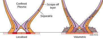
6 Fluid description of plasma : Assumptions Macroscopic velocity is small compared to the sound speed or magnetic speed (Alfen) [ ] [ ] γp b [v] [v] ρ ρ Deby lenght is small compared to characteristic system lenght: local electrical quasi-neutrality Te n e e 2 [x] Magnetic speed is small compared to light speed : negligible displacement current [ ] b c l ρ ν = ν ei ω b 1 where ω b = T e m e 1 q(r)r

7 Fluid description of plasma : MHD equations Rationalized Gaussian unit (c=1) Conservation of particles Conservation of momentum (ions + elect.) Conservation of energy (ions &/+ elect.) Faraday s law t ρ + m = m t m + (m v) + (pi + πi b b) = (τ + τ ) t E + ((E + p π) v + e b) + q = (( τ + τ ) v ) t b + e = 0 Conservation of elect. momentum (generalized Ohm s Law ) Ampere s law { e = v b + ηj + ẽ j = b

8 Fluid description of plasma : MHD equations Rationalized Gaussian unit (c=1) Spitzer 1956 : Ion Larmor radius [R i ] = ẽ = 1 n e e p i + m e n e e 2 tj + m i e tv [ẽ] = [R i ] [x] Ma + 1 ω p [t] + 1 ω l [t] 2mi [T i ] [b]e [ne]e 2 Plasma frequency ω p = m e Ion Larmor frequency ω l = [b]e m i Mach number Ma = [v] [c] For Equilibrium without flow Ma 1

9 MHD : Fluid description of plasma Conservative formulation : t ρ + m = m t m + (m v) + (pi + πi b b) = (τ + τ ) t E + ((E + p π) v + e b) + q = (( τ + τ ) v ) t b + e = 0 Closure relations : 1 m = ρv 2 E = ρε + ρ v v 2 + b b 2 3 p = (γ 1)ρε 4 π = b b 2 5 e = v b + ηj + ẽ 6 j = b ẽ contains the inductive applied electric field.

10 MHD : pressure formulation t ρ + m = m t m + (m v) + (pi + πi b b) = τ + τ t p + v p + ρc 2 v = (γ 1) q t b + e = 0

11 Constraint No magnetic monopole : b = 0 Divergence free current : j = 0 Potential Vector formulation b = a Implies that { { ( a) = 0 ( a) = 0 = h ( h a h ) = 0 h ( h h a h ) = 0 Constraints contains third order derivatives!

12 Numerical Strategy : Jorek System of equations in compact form : t w = L (, w) C1-Finites elements ( h a h ) ( h ( h ϕ) ) = 0 Implicit scheme for MHD instabilities (Elm s).

13 Taylor Galerkin Principle of the TG Method (LW, Donea(84)) Formulate a high-order time-stepping scheme algorithm before the discretization of the spatial variable w n+1 = w n + δt ( t w) n (δt)2 ( 2 t w ) n (δt)3 ( 3 t w ) n + Substitute time derivatives by space derivatives: ( t w) n L (, w n ), ( k+1 t w ) n ( k t L (, w) ) n Solve the PDE with δw = w n+1 w n δw δt = L (, wn ) δt 2 ( tl (, w) ) n (δt)2 ( 2 6 t L (, w) ) n

14 Stabilization TG2/TG3 Ambrosi & Quartapelle JCP(98) w n+1 = w n + δt ( t w) n (δt)2 ( 2 t w ) n (δt)3 ( 3 t w ) w n+1 w n = δt ( t w) n (δt)2 ( 2 t w ) n (δt)3 ( 3 t w ) Approximation : ( t 3 w ) ( 2 3β t w ) n+1 ( 2 t w ) n δt General form : 0 θ 1 and 0 β 1 δw δt + θ ( L (, w n+1) L (, w n ) ) + δtξ l (( ) 2 t L) n+1 ( t L) n = L (, w n ) δtξ e 2 ( tl) n where ξ l = θ β and ξ e = 2θ 1.

15 Stabilization TG2/TG3 1 This is third order accurate only when β = Second order accurate for others values. Linear hyperbolic : L (, w) = (A ) w = a w t L (, w) = a ( tw) = 2 a w δw δt + θl (, w n+1) δtξ l 2 2 a a wn+1 = (θ 1)L (, w n ) + δt(ξ e ξ l ) 2 Crank-Nicolson scheme : θ = 1/2 and β = 1/2. In this case ξ l = ξ e = 0 2 a wn

16 Stabilization TG2/TG3 :Linearized hyperbolic component. L (, w) (A ) w + L re (, w). { ( t L) n+1 ( t L) n ( a R n+1 ) ( t L) n a (Rn ) 0 + a tw n 1 where R k+1 = ( t w) k + L (, w k+1) wk+1 w k t k+1 t k + L (, w k+1) δw δt + θ ( L (, w n+1) L (, w n ) ) δtξ l 2 ( a R n+1 ) = L (, w n ) + δtξ e 2 a (Rn )

17 Application to Full MHD t w+l (, w) = 0 with w = where L ρ (, w) = (ρv) (D ρ) ρ m p b, L (, w) = L ρ (, w) L m (, w) L p (, w) L b (, w) L m (, w) = (ρv v + pi + πi b b) + π ( ) L p (, w) = v p + γp v Γ (λ T ) + π : v + ηj j L b (, w) = e

18 Application to Full MHD We are concerned by plasmas dynamically dominated by ideal MHD pattern : L (, w) = L (, w) + L re (, w) with ( m ) m m L (, w) = ρ + pi + πi b b v ( p + γp v ) m b ρ b m ρ Then L (, w) = ÃA (w, ) w with 0 t 0 0 (v v) v + v (b ) t b ÃA (w, ) = γp ρ v γp ρ t v 0 vb bv b ρ ρ 0 v Taylor-Galerkin method is defined with A e = ÃA (w n e, )

19 Simplified semi-implicit and Implicit stabilizations = a ( i δtξ l δw a Rn+1 a δt and a Rn 0 ) δw 2 a δt + θl (, w n+1) = (1 θ) L (, w n )

20 Simplified semi-implicit and Implicit stabilizations The Harned and Kerner algorithm : θ = 0 and a = ÃA (w n, ) 0 t 0 0 δρ 0 0 (b ) t δt δtξ l δm 2 t ( δt ) = L ρ ( δm δt à (w, ) = δtξ l 2 δp δt + (bn ) t δb δt = L m ( ) γp δp 0 ρ t 0 0 δt δtξ l γp n 2 ρ t δm n δt = L p ( ( ) δb b 0 ρ 0 0 δt δtξ l b n δm 2 ρ n δt = L b ( Self consistent implicit scheme for the momentum: ( ( ) ) 2 δtξl i G (w n δm, ) 2 δt = L m (, w n ) δtξ l 2 K (, wn ) (1) where G (w n, ) is a self-adjoint (in (L 2 ) 3 ) linearized operator associated to ideal MHD ( ) ( ) γp G (w n n, ) = + (b n ) t 1 ρ n bn ρ n t

21 Ritz-Galerkin method for MHD. Approximated weak stabilized(taylor-galerkin) formulation t ρ h ρ h = L ρ,h (, w h ) ρ h δt t L ρ,h (, w h )ρ h 2 t m h m h = L m,h (, w h ) m h δt t L m,h (, w h ) m h 2 t E h Eh = L E,h (, w h ) Eh δt t L E,h (, w h )Eh 2 t b h b h = L b,h (, w h ) b h δt t L b,h (, w h )b h 2 Test functions : ρ h, m h, E h and b h. For any scalar variable defined over a domain Ω x, V h V h ( ) is the approximated space of function (of finite dimension) to be defined. Ritz-Galerkin formulation ρ h V h, m h (V h ) d, E h V h and b h (V h ) d ρ h V h, m h (V h ) d, Eh V h and b h (V h ) d What about the divergence free condition : b = 0?

22 Ritz-Galerkin method for MHD. Approximated weak stabilized(taylor-galerkin) formulation t ρ h ρ h = L ρ,h (, w h ) ρ h δt t L ρ,h (, w h )ρ h 2 t m h m h = L m,h (, w h ) m h δt t L m,h (, w h ) m h 2 t E h Eh = L E,h (, w h ) Eh δt t L E,h (, w h )Eh 2 t b h b h = L b,h (, w h ) b h δt t L b,h (, w h )b h 2 Ritz-Galerkin formulation ρ h V h, m h (V h ) d, E h V h and b h (V h ) d ρ h V h, m h (V h ) d, Eh V h and b h (V h ) d Ritz-Galerkin formulation with potential vector ρ h V h, m h (V h ) d, E h V h and b h F eq φ + (V h ) d ρ h V h, m h (V h ) d, E h V h and b h?? F eq φ + (V h ) d

23 Well Balanced scheme m h V h φ V h r V h ẑz (V h ) d m h V h b h V h r V h ẑz (V h ) d

24 Reduced Resistive MHD: b = F eq φ + (ψ φ) Therefore the induction equation becomes ( t ψ φ + e) = 0 so that t ψ φ + e = (F 0 u + u eq ) where F 0 (constant) is the scale of F eq e = v b + η (j j eq ) + u eq + ẽ Then v b = t ψ φ + η (j j eq ) + ẽ F 0 u Projections of this equation give: { t ψ = r2 F eq b (F 0 u η (j j eq ) ẽ ) v ϑb = 1 ( b b F 0 u η (j j eq ) ẽ t ψ φ ) b Tokamaks Scaling of the drift velocity: v ϑb r 2 u φ Why not v ϑb F 0 b b u b to enfore the relation b (v ϑb) = 0?

25 Reduced MHD : Elms Scale v = ϑb + r 2 u φ and b = F eq φ + (ψ φ) Ritz-Galerkin formulation for Reduced MHD ρ h and ρ h V h E h and E h V h m h and m h V h b h + r 2 V h φ b h F eq φ + V h φ and b h?? F eq φ + V h φ ( ) Simplified stabilization : a 2 τ ϑ where w = F eq r φw + [w, ψ] and w = r 2 [w, u]

26 Momentum equation : m h and m h V h b h + r 2 V h φ ( ϕb h ϕ φ ) 2 tl m,h (, w h ) ( (r 2 t m h + L m,h (, w h ) + δt ) ) 2 tl m,h (, w h ) t m h + L m,h (, w h ) + δt = 0 = 0 ϕ V h Conservative formulation 1 L m,h (, w h ) O h + β h β h = p h + π h 2 t L m,h (, w h ) t O h + t β h Tokamak scaling near equilibrium 1 β h = β h + 1 ɛ β h O h = ρ hv h v h 2 O h = O h + 1 ɛ O h O h = b h b h

27 Reduced MHD : Induction equation t ( ψ r 2 ) ϕ = φ ( e) ϕ formally implies, with j φ = ψ, that ( ) jφ t r 2 + φ ( e) = 0 ϕ V h

28 C1-Quadrangles Finite element (1) ϕ j (s, t) (2) ϕ j (s, t) (3) ϕ j (s, t) (4) ϕ j (s, t)

29 C1-Triangles Finite element

30 Tokamak s Equilibrium Ohm s Law e = v b + η (j j eq ) + u eq + ẽ It is often assumed that u eq 0 and ẽ 0. Grad-Shafranov Equilibrium: b eq = F eq φ + (ψ eq φ) where F eq F (ψ eq ) and p eq p (ψ eq ) are precribed functions, by solving ψ = F (ψ) F p (ψ) + r2 ψ ψ

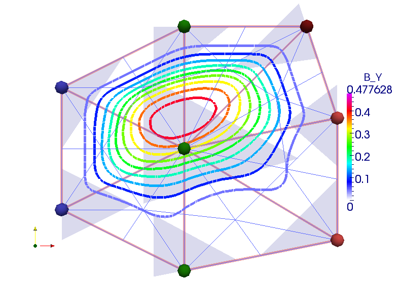
31 Triangular mesh aligned with the magnetic surfaces. From Vtx and Elmt to 4000 Vtx and 8000 Elmt

32 Triangular mesh aligned with the magnetic surfaces.

33 Triangular mesh aligned with the magnetic surfaces.

34 Triangular mesh aligned with the magnetic surfaces.

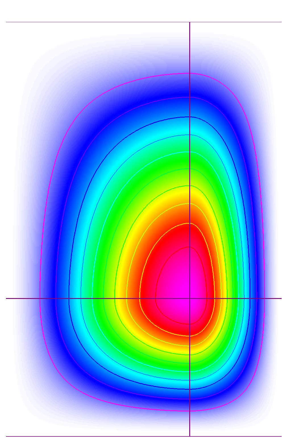
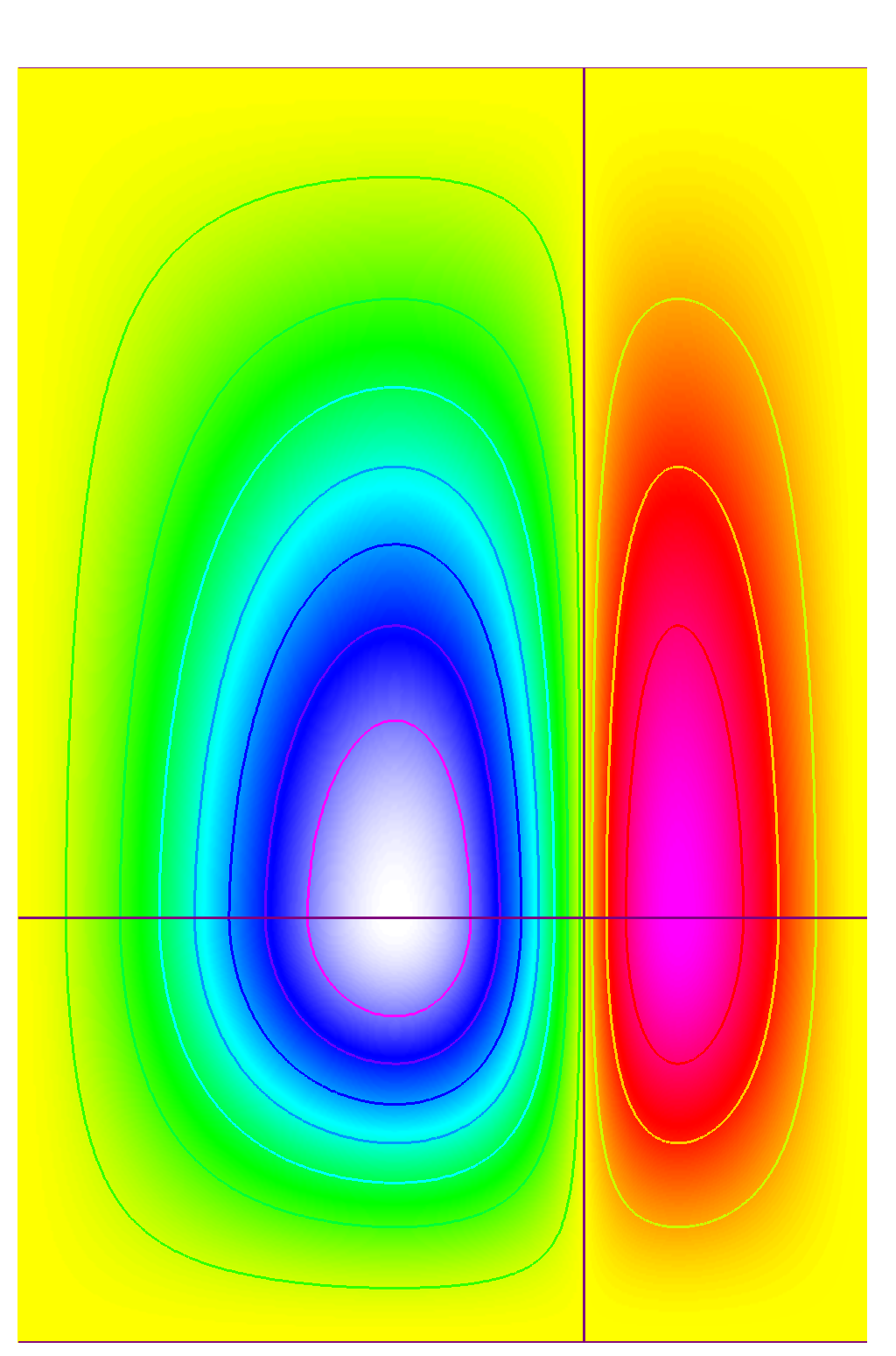
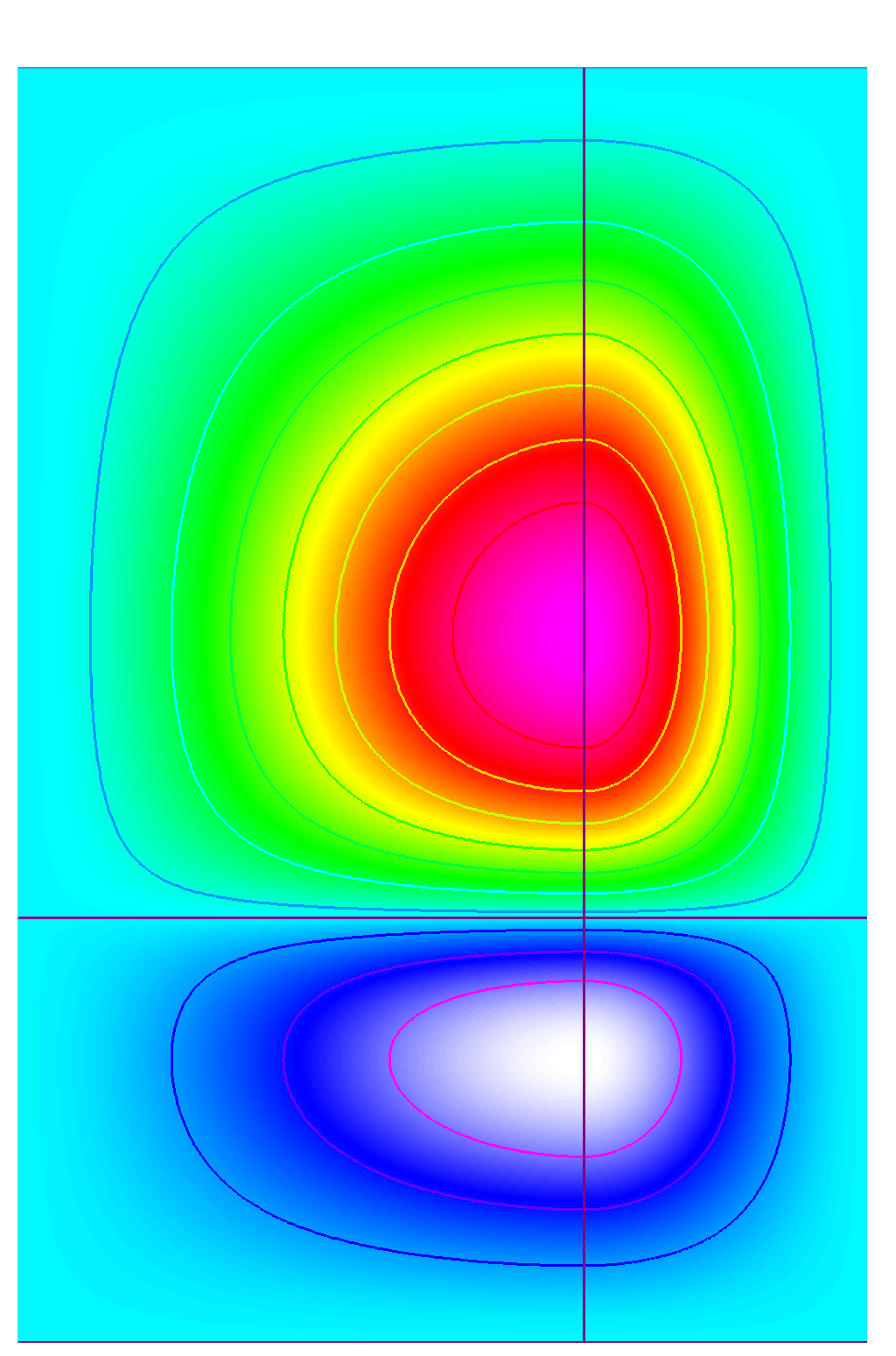
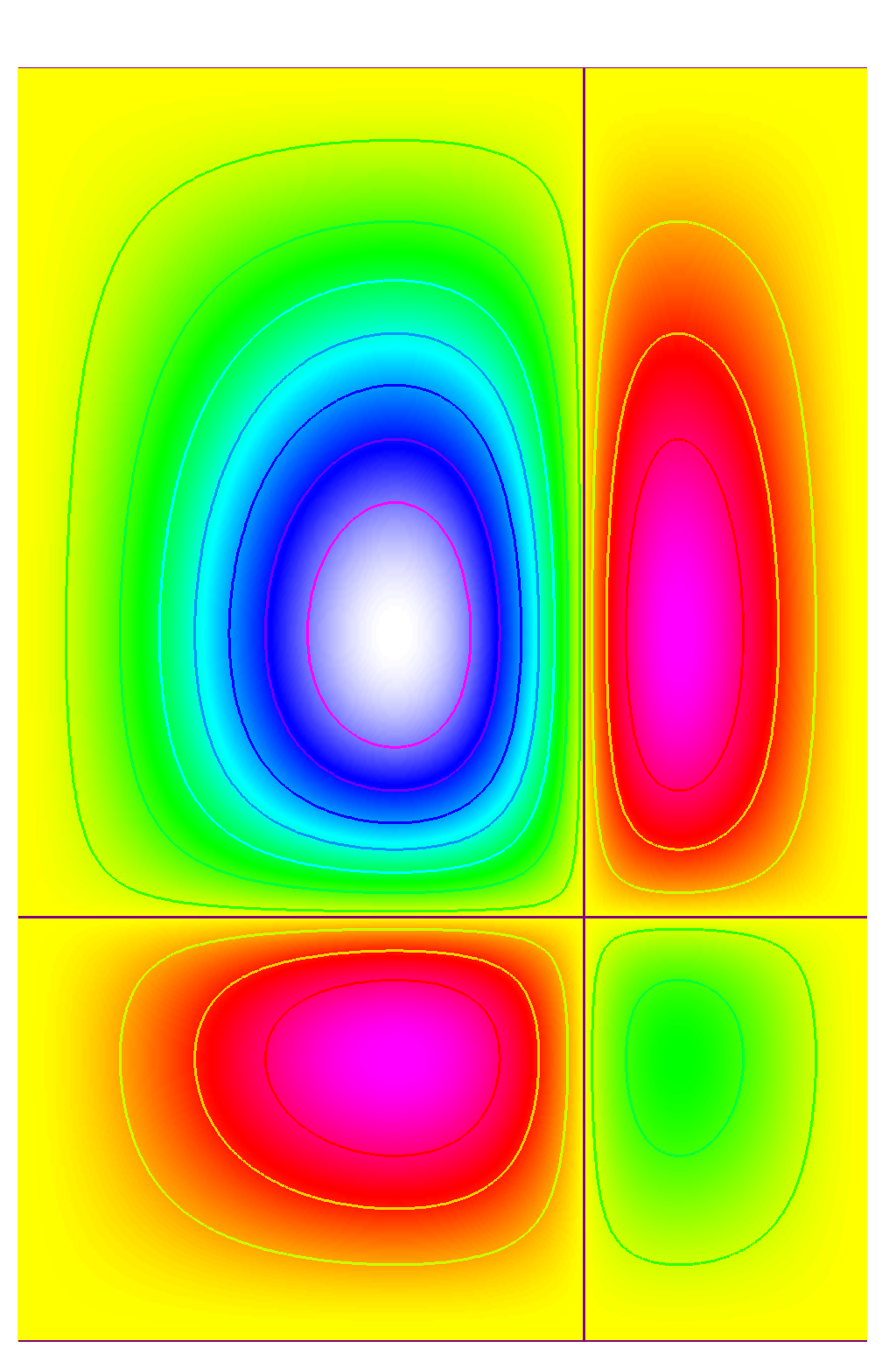
35 Internal kink Grow rate

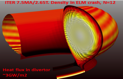
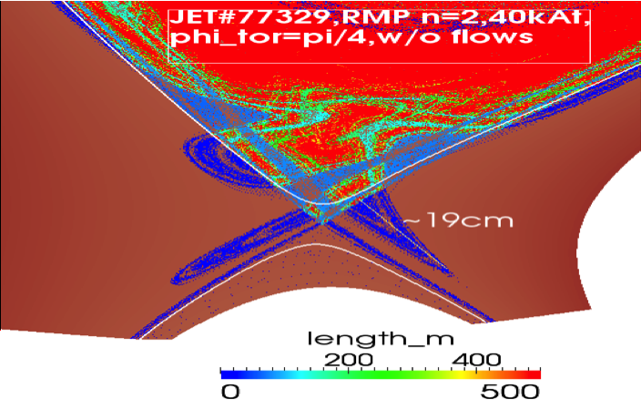
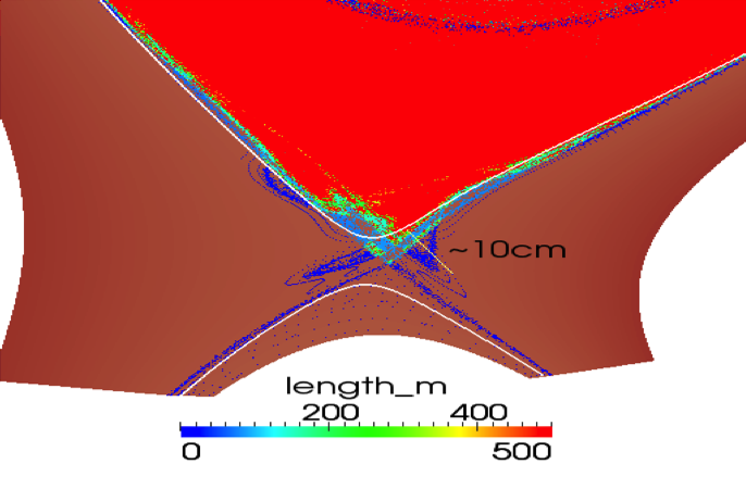
36 ELM s control by RMP.

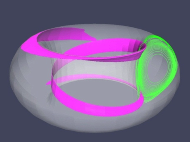
37 ELM s control by Pellet.

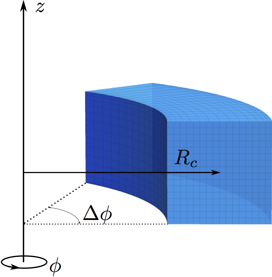
38 Conclusion Toroidal Finite Element Powell-Sabin Poloidal FE (Triangles) Improved Stabilization and Full MHD Modeling TR-BDF2 : second-order accurate and L-stable : lim δt 0 w n+1 w n = 0. Large-scale computations