Diamond platforms for nanoscale photonics and metrology
|
|
|
- Σώστρατος Αλαφούζος
- 7 χρόνια πριν
- Προβολές:
Transcript
1 Diamond platforms for nanoscale photonics and metrology The Harvard community has made this article openly available. Please share how this access benefits you. Your story matters. Citation Accessed Citable Link Terms of Use Shields, Brendan John Diamond platforms for nanoscale photonics and metrology. Doctoral dissertation, Harvard University. December 30, :35:42 PM EST This article was downloaded from Harvard University's DASH repository, and is made available under the terms and conditions applicable to Other Posted Material, as set forth at (Article begins on next page)
2
3
4
5
6
7
8 594
9
10
11
12
13
14
15
16
17
18 0 637 m s =0 m s = ±1 2.8 m s = ±1 m s =0 m s =1 m s = ±1 m s = ±1 150 m s = 0 m s = 1 m s =0
19
20 532 m s =0 V Q V (λ/n) 3 λ n
21 2π 15
22 2π Q n = 2.4 Q
23
24
25
26 V m 1/ V m Q ΓX

 g.. onto substrate.")
 normalized frequency a/h a V PC tip 0 film 1")
 6B;m`2 kxr, U V.BbT2`bBQM 7Q` i?2 T?")


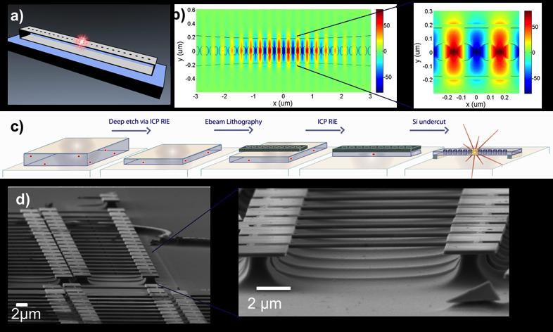
27 air 0.3 light -lines PMMA e d waveguide bands bandgap X J k a// x E Air 2 z(+m) ï 1 1 b 1 5+m f 4 Target NV N h(nm) g.. onto substrate. 30+m 1+m 0.2..to polymer.. GaP wafer.. intensity (a.u.) normalized frequency a/h a V PC tip 0 film 1 PMMA c glass y(+m) ï 0 excitation & collection ï ï 0 x(+m) 6B;m`2 kxr, U V.BbT2`bBQM 7Q` i?2 T?QiQMB+ +`vbi H bh # BM B`- HQM; i?2 r p2;mb/2 /B`2+iBQM kx c i?2 BMb2i b?qrb i?2 +`vbi H UQ` M;2V M/ BMp2`b2 +`vbi H U#Hm2V /B`2+iBQMbX h?2 H iib+2? b T2`B@ Q/B+Biv Q7 a = 176MK-?QH2 ` /Bmb Q7 53 MK- M/ bh #?2B;?i Q7 110 MKX U#V 1M2`;v /2MbBiv 7Q` 7mM/ K2Mi H KQ/2 BM +`Qbb@b2+iBQM M/ U+V BM TH M2X U/V a1jx U2V h?2 T?QiQMB+ +`vbi Hb `2 i` Mb72``2/ 7`QK i?2 : S +?BT QMiQ bm#bi` i2 pb TQHvK2` bi KTX U7V "`Q /@# M/ `2~2+iBpBiv K2 bm`2k2mi Q7 + pbiv `2bQM M+2 rbi? Q X U;V h?2 S* bh # Bb TQbBiBQM2/ `2H ibp2 iq i `;2i M MQ+`vbi H BM i?2 TQHvK2` }HKX Rk
28 n s 1.5 Q V m =0.74(λ/n ) 3 n =3.4 λ = Q Q 30
 g (t ) 1 (2) g (t ) 0 620 640 660 680 700 720 1 1 0.5 0 1 0.")
 500 0.2 I 0 I cb I c f c (λ 2 ) = 5.3,f c (λ 1 ) = 0.")
29 a y(µm) b PL reflection x(µm) NV c 100 cts/s/nm 100 cts/s/nm cavity and NV d 4 2 I 0 I cb fits I c 2 2 (2) g (t ) 1 (2) g (t ) λ(nm) t (ns) t (ns) intensity (a.u.) e f uncoupled, τ =16.4 ±1.1 ns 0 coupled, τ =12.7 ± 1.2 ns c t(ns) I 0 I cb I c f c (λ 2 ) = 5.3,f c (λ 1 ) =
30 λ 1 = λ 2 = Q 1 = 550 Q 2 = I I c I cb
31 τ 0,c = 16.4 ± 1.1, 12.7 ± 1.5 F (λ) F (λ) =I c (λ)τ 0 /I 0 (λ)τ c F (λ 1 )=2.2 F (λ 2 ) 7.0 F (λ) a 180 S d (ω, r) =C NV + C cav f c ( r ) L(ω) 2 +2C int R[e i φ f c ( r )L(ω)], C NV C cav C int L(ω) =1/(1 + i(ω ω c )/κ) ω c κ = ω c /2Q φ

 fits 635")


 x = 3.")
32 a target NV b c e target NV 4 µm scanning tip x d 1 µm PL reflection 680 λ λ 2 f PL λ(nm) fits x(nm) g experiment c f (λ, x x+ y ^ y) ^ 1 slip theory 0.3 y(µm) 0 y(nm) 0.3 c ^ h f (λ, x x+ y ^ y-98 ^ o 1 nm z, 20 ) x(nm) x = 3.4 f c (λ 1, r) 80 f c (λ 1, r) z = 98 ± 5 y = 70 ± 5 µ x
33 f c (ω, r) C NV C cav C int C NV C cav C int C int =0 f c (λ = 643, r)=5.3,f c (667, r)=0.7 S d (ω, r) f c (ω 1, r) ω 1 =2πc/λ 1 f c (ω 1, r) µ z = 98 ± 5 20 x x 190
34
35
36
37
38 Q 7 23
39 n =2.4

40 Q Q
41 T Q 2 Tot /Q2 wg Q Q scat Q Q wg Q Q Tot (λ/n) 3 Q Q scat = <Q wg 3.7(λ/n) 3 Q
42 Q Q Q

43 532 g 2 (0) =
44 23 7 Q
45 23
46 Q Q
47 F P 7
48 F P = 3 4π 2 ( ) λ 3 Q n V E NV µ NV 2 E max 2 µ NV 2, E NV,max µ NV λ n = 2.4 V = [ ɛ( r ) E( r ) d r] 2 /max [ɛ( r ) E( r ] ) I res ZPL =(η cav F P + η NV ) 1 τ 0, η cav,nv τ 0
49 F P =0 I off res ZPL = η NV F NV τ 0. η cav = η NV Q ZPL I off res ZPL χ = η cavf P η N V = Ires 1. χ Q 3.7 (λ/n) 3 Q Q 23 7
50 Q 10 3
51 0 0
52 0 m s =

53
54 n diamond n glass 532 m s = ±1 25 m s =0 m s =1
55 g 1 g 0 0 γ 0 γ 1 F C g 0,1 γ 0,
56 594 0 γ 1 γ 0 g 1 g µ γ 0,γ 1,g 0,g 1 594
57 15 t tg 1 1 P t R F C (P ) F C 0.9 µ t probe = g 1 t probe 1 t R = ± 0.006
58 0.975 ± p s =0.216 ± m s =1 m s =0 594 m s = 1 m s = m s =0 m s =
59 ± p s =0.216 ± ±
60 m s =0 m s = m s =0 0 m s = m s = ± m s = ±
61 m s = 0 m s =1 β 0 β 1 β 0 β 1 β 0,1 β 0,1 20 β 0,1 m s =1 β 1 60 δb = π τ + ti + t R σ R 2gµ B T τ 2, g µ B τ t I t R T N τ + t I + t R σ R
62 σ R t R m s =0 m s = t R σ R (t R ) = a 1+b/t 1/4 R a b t R σ R (t R ) σ R (t R ) (τ + t I + t R )/τ 2 t I 6.5 t I =1.5/p s p s =0.200 ± 0.006
63 σ R =1 τ α 0,1 m s =0, 1 σ trad R = 1+ 2(α 0 + α 1 ) (α 0 α 1 ) 2 σ trad R α 0 20 = ± α 1 =0.154 ± σ trad R = 10.6 ± 0.3 σ SCC R = (β 0 + β 1 )(2 β 0 β 1 ) (β 0 β 1 ) 2.
64 β 0,1 σ SCC R,best =2.76 ± 0.09 σr SCC (t R ) 6.5 t R σr SCC (t R ) β 0,1 t R σr SCC (t R ) t R 5 σr SCC (t R ) σr SCC (t R ) σr SCC (t R ) σ SCC R,best (t R) δb T = π τ + 2gµ ti + t R σscc R (t R ) τ 2
65 t R σr SCC (t R ) t R = /2 0
66
67 Q 10 5 Q
68
69
70 N j λ j γ j γ NR r i p i j I ij = cp i η ij γ ij k γ ik + γ NR = cp i η ij γ ij Γ i
71 η ij Γ i = k γ ik + γ NR c β ij = γ ij /Γ i j Γ i =1/τ i i 0 I ij I 0j = p iη ij γ ij Γ 0 p 0 η 0j γ 0j Γ i I ij I 0j = γ ijγ 0 γ 0j Γ i = F ij Γ 0 Γ i, F ij = γ ij /γ 0j = I ij Γ i /I 0j Γ 0 i =1 F 1j = F (λ j )
72 a b 80 cts/s/nm cts/s/nm 2 uncoupled NV uncoupled cav. 1 coupled NV/cav. fits x(nm) c Scan over NV centre λ(nm) fit λ(nm) C int =0.6 x 1 x 2 x x 1 λ 1 λ 2 λ 2
73 F(λ) λ(nm) F (λ)
")
 100 80 60 40 20 d intensity")
74 a.1 λ 2 pump a.2 λ 2 a.3 λ 1, y-polarized, x-polarized, y-polarized y x(nm) x(nm) x1 x2 b c degrees λ 2 λ 1 collection from x2 collection from x λ(nm) d intensity (cts/s/nm) λ(nm) λ 1
75 C int = 0.6 = 2.87 m s = 0 m s = ±1 m s = ±1 m s = ±1 m s =0 m s = ±1
76 (2) g (τ) τ(ns)
77 Luminescence intensity (a.u.) 7 (a) Luminescence intensity (a.u.) (b) ν(ghz) microwave frequency t(ns) microwave pulse duration ν ν =2.77 ν m s =0 t ν =2.77 σ = g e a H = 2 a a 2 (σ z)+ig(σa aσ ),
78 dρ dt = i[h, ρ]+κ 2 (2aρa a aρ ρa a)+ γ 2 (2σρσ σ σρ ρσ σ)+ γ d 2 (σ zρσ z ρ) γ κ γ d σ z =[σ,σ] g, e 0, 1. da =( i dt 2 κ ) a + g σ 2 dσ =(i dt 2 γ 2 γ d) σ + g σ z a a(0) = 0,σ(0) = 1 σ z a = a c 1 = ( i 2 κ 2 ) c2 = ( i 2 γ 2 γ d) λ = c 1 +c 2 (c 1 c 2 ) 2 4g 2 λ + = c 1 +c 2 + (c 1 c 2 ) 2 4g 2 a(t) = (eλ +t e λ t )g (c1 c 2 ) 2 4g 2 σ(t) = (c 1 c 2 )(e λ t e λ +t )+ (c 1 c 2 ) 2 4g 2 (e λ t + e λ +t ) 2 (c 1 c 2 ) 2 4g 2
79 E (+) = γσê NV + κaê c + c.c., ê NV ê c ˆf( k, ω) E + = U F ( γσê NV + κaê c ), U F = k,ω ( ˆf( k, ω))( ˆf( k, ω) ) S(ω) 0 E + (t)e (t ) dtdt ω = ω c,κ γ d,g γ d,κ S (ω) ê NV U F ê NV +2R[ê NV U F ê c e i φ f c 1 ( r ) 1+i(ω ω c )/κ ]+ ê c U F ê c f c 1 ( r ) 1+i(ω ω c )/κ 2, F =(g( r, µ )) 2 /κγ r µ / µ ê NV U F ê c S d (ω) =C 1 +2C 2 R[e i φ f c 1 ( r ) 1+i(ω ω c )/κ ]+C 3f c 1 ( r ) 1+i(ω ω c )/κ 2,
80 C i C 2 /C C 2 /C 1 0 PL(ω, r) e( r ) PL(ω, r) = e( r r )S d (ω, r )dl dl r PL(ω, r) = S d (ω, r) e ( r ) PL ( r ) S d (ω, r ) e ( r )
81
82
83 9 F (τ) =A + Be (τ/t 2) n e ((τ jtrev)/t dec) 2, j=0 A =0.844 ± B =0.143 ± n =1.72 ± 0.14 T rev = ± 0.04µ T dec =7.47 ± 0.22µ T 2 = 201 ± 7µ 0 g 1 g 0 0 γ 1 γ 0 γ 1,0 0 τ 1 t 1 γ 1 (t R t 1 )+γ 0 t 1 t R p(n NV, odd) = tr 0 i 1 j=1 dτe (g 0 g 1 )τ g 0 t R (tr τ) (j 1) k=1 t k 0 i=1 g i 1g i 1 0 i 1 j=1 τ (j 1) k=1 τ k 0 ds j dt j PoissPDF(γ 1 τ + γ 0 (t R τ),n)
84 p(n NV, even) = tr 0 i 1 j=1 dτe (g 0 g 1 )τ g 0 t R (tr τ) (j 1) k=1 t k 0 i=1 (g 1 g 0 ) i i j=1 τ (j 1) k=1 τ k 0 dτ j dt j PoissPDF(γ 1 τ + γ 0 (t R τ),n) +e g 1t R PoissPDF(γ 1 t R,n) τ [0,t R ] PoissPDF(x, n) n x p(n NV, even) i p(n NV, odd) = p(n NV, even) = tr 0 tr 0 dτg 1 e (g 0 g 1 )τ g 0 t R BesselI(0, 2 g 1 g 0 τ(t R τ)) g1 g 0 τ dτ t R τ e(g 0 g 1 )τ g 0 t R BesselI(1, 2 g 1 g 0 τ(t R τ)) +e g 1t R PoissPDF(γ 1 t R,n), BesselI(n, x)
85 F C T 1/g 1 (P ) 594 P T T g 1 g 0,1 g 0 /g 1 = p(nv )/p(nv 0 ) a P/(1 + P/P sat )+dc P sat dc ap 2 /(1 + P/P sat ) P sat
86 594 g 0 ap 2 /(1 + P/P sat ) P sat = 134 a = 39 µ 2 g 1 ap 2 /(1 + P/P sat ) P sat = 53.2 a = 310 µ 2 γ 0 a P/(1 + P/P sat )+dc dc =0.268 a =1.65 µ P sat = 134 γ 1 a P/(1 + P/P sat )+dc a = 46.2 µ P sat = 53 γ 0,1 g 0,1
87 F C n thresh =[1, 2, 3] F C F C (P, t R ) n n thresh NV n<n thresh NV 0 t R n thresh =[1, 2, 3] m s =0 t I τ t R
88 N T = N(τ + t I + t R ) ( gµb Bτ ψ(τ) = cos π ) m s =0 i sin ( gµb Bτ π ) m s =1, g g B m s =0, m s =1 ( ) p 0 = cos 2 gµb Bτ π p 1 = 1 p 0 =sin 2 ( gµb Bτ π ). D 0 (n) D 1 (n) ψ(τ) P (n) =p 0 D 0 (n)+p 1 D 1 (n). δb S = n σ S δb = σ S S/ B = π gµ B τ σ S D 0 D 1,
89 p 0 = p 1 =1/2 N 1/ N σ R δb = π τ + ti + t R σ R 2gµ B T τ 2. = 2gµ Bτ π σ S S/ B σ R =1 σ R t I t R σ R σ R m s =0 m s =1 β 0 m s =0 β 1 m s =1 D 0 (n) D (n) 0 π 2gµ B =8.9 1
90 D D 0 σd 2 σ 2 D 0 P (n) =p 0 (β 0 D (n)+(1 β 0 )D 0 (n)) + (1 p 0 )(β 1 D (n)+(1 β 1 )D 0 (n)) σ R p 0 = p 1 =1/2 σr SCC = 2gµ Bτ σ S π S/ B S = p 0 (β 0 D +(1 β 0 ) D 0 )+(1 p 0 )(β 1 D +(1 β 1 ) D 0 ) = β ( 0 + β 1 D + 1 β ) 0 + β 1 D S B = gµ Bτ π (β 0 β 1 )( D D 0 ) [ ] σs 2 = n 2 P (n) S 2 σ SCC R = n=0 = 1 4 (β 0 + β 1 )(2 β 0 β 1 )( D D 0 ) 2 + β ( 0 + β 1 σd β ) 0 + β 1 σ 2 D (β 0 + β 1 )(2 β 0 β 1 ) (β 0 β 1 ) σ2 D /(2 β 0 β 1 )+σ 2 D 0 /(β 0 + β 1 ) ( D D 0 ) 2
91 σ R D (n) D 0 (n) σ SCC R (β 0 + β 1 )(2 β 0 β 1 ) (β 0 β 1 ) 2. β 0 β 1 m s =0 m s =1 σ R β 0,1 m s =0 m s =1 β 0,1 σr SCC (t R ) σ SCC R t R t R σr SCC
92 σr SCC σr SCC (t R ) D D 0 D (n) σ D D γ 1 t R σ SCC R (β 0 + β 1 )(2 β 0 β 1 ) 2 (β 0 β 1 ) (2 β 0 β 1 )γ 1 t R γ 1 t 3/4 σ SCC R σ SCC R = a 1+b/t 1/4 a =1.328 b = 39.3 a σr,best SCC
93
94
95
96 ɛ
97
98
99
100
101
102
Defects in Hard-Sphere Colloidal Crystals
 Defects in Hard-Sphere Colloidal Crystals The Harvard community has made this article openly available. Please share how this access benefits you. Your story matters. Citation Accessed Citable Link Terms
A Classical Perspective on Non-Diffractive Disorder
 A Classical Perspective on Non-Diffractive Disorder The Harvard community has made this article openly available. Please share how this access benefits you. Your story matters. Citation Accessed Citable
Gradient Descent for Optimization Problems With Sparse Solutions
 Gradient Descent for Optimization Problems With Sparse Solutions The Harvard community has made this article openly available. Please share how this access benefits you. Your story matters Citation Chen,
Note: Please use the actual date you accessed this material in your citation.
 MIT OpenCourseWare http://ocw.mit.edu 6.03/ESD.03J Electromagnetics and Applications, Fall 005 Please use the following citation format: Markus Zahn, 6.03/ESD.03J Electromagnetics and Applications, Fall
 www.smarterglass.com 978 65 6190 sales@smarterglass.com &&$'()!"#$%$# !!"# "#$%&'! &"# $() &() (, -. #)/ 0-.#! 0(, 0-. #)/ 1!2#! 13#25 631% -. #)/ 013#7-8(,83%&)( 2 %! 1%!#!#2!9&8!,:!##!%%3#9&8!,:!#,#!%63
m i N 1 F i = j i F ij + F x
 N m i i = 1,..., N m i Fi x N 1 F ij, j = 1, 2,... i 1, i + 1,..., N m i F i = j i F ij + F x i mi Fi j Fj i mj O P i = F i = j i F ij + F x i, i = 1,..., N P = i F i = N F ij + i j i N i F x i, i = 1,...,
14.5mm 14.5mm
 This article has been accepted for publication in a future issue of this journal, but has not been fully edited. Content may change prior to final publication. Citation information: DOI 1.119/JETCAS.218.289582,
Physique des réacteurs à eau lourde ou légère en cycle thorium : étude par simulation des performances de conversion et de sûreté
 Physique des réacteurs à eau lourde ou légère en cycle thorium : étude par simulation des performances de conversion et de sûreté Alexis Nuttin To cite this version: Alexis Nuttin. Physique des réacteurs
ITU-R P (2012/02) &' (
 &' (") ITU-R P.530-4 (0/0) $ % " "#! &' ( P ITU-R P. 530-4 ii.. (IPR) (ITU-T/ITU-R/ISO/IEC).ITU-R http://www.itu.int/itu-r/go/patents/en. ITU-T/ITU-R/ISO/IEC (http://www.itu.int/publ/r-rec/en ) () ( ) BO BR BS
ITU-R P.530-4 (0/0) $ % " "#! &' ( P ITU-R P. 530-4 ii.. (IPR) (ITU-T/ITU-R/ISO/IEC).ITU-R http://www.itu.int/itu-r/go/patents/en. ITU-T/ITU-R/ISO/IEC (http://www.itu.int/publ/r-rec/en ) () ( ) BO BR BS
APPLICATIONS TECHNOLOGY. Leaded Discs N.03 N.06 N.09
 NC Disc hermistors ND 03/06/09 NE 03/06/09 NV 06/09 APPLICAIONS ND or NE: Commerical, Industrial and Automotive Applications AEC-Q200 Qualified NV: Professional Applicationsl Alarm and temperature measurement
!!" #7 $39 %" (07) ..,..,.. $ 39. ) :. :, «(», «%», «%», «%» «%». & ,. ). & :..,. '.. ( () #*. );..,..'. + (# ).
 ..,..,.. $ 39. ) :. :, «(», «%», «%», «%» «%». & ,. ). & :..,. '.. ( () #*. );..,..'. + (# ).") 1 00 3 !!" 344#7 $39 %" 6181001 63(07) & : ' ( () #* ); ' + (# ) $ 39 ) : : 00 %" 6181001 63(07)!!" 344#7 «(» «%» «%» «%» «%» & ) 4 )&-%/0 +- «)» * «1» «1» «)» ) «(» «%» «%» + ) 30 «%» «%» )1+ / + : +3
1 00 3 !!" 344#7 $39 %" 6181001 63(07) & : ' ( () #* ); ' + (# ) $ 39 ) : : 00 %" 6181001 63(07)!!" 344#7 «(» «%» «%» «%» «%» & ) 4 )&-%/0 +- «)» * «1» «1» «)» ) «(» «%» «%» + ) 30 «%» «%» )1+ / + : +3
Jeux d inondation dans les graphes
 Jeux d inondation dans les graphes Aurélie Lagoutte To cite this version: Aurélie Lagoutte. Jeux d inondation dans les graphes. 2010. HAL Id: hal-00509488 https://hal.archives-ouvertes.fr/hal-00509488
Parts Manual. Trio Mobile Surgery Platform. Model 1033
 Trio Mobile Surgery Platform Model 1033 Parts Manual For parts or technical assistance: Pour pièces de service ou assistance technique : Für Teile oder technische Unterstützung Anruf: Voor delen of technische
Q1a. HeavisideTheta x. Plot f, x, Pi, Pi. Simplify, n Integers
 2 M2 Fourier Series answers in Mathematica Note the function HeavisideTheta is for x>0 and 0 for x
 W τ R W j N H = 2 F obj b q N F aug F obj b q Ψ F aug Ψ ( ) ϱ t + + p = 0 = 0 Ω f = Γ Γ b ϱ = (, t) = (, t) Ω f Γ b ( ) ϱ t + + p = V max 4 3 2 1 0-1 -2-3 -4-4 -3-2 -1 0 1 2 3 4 x 4 x 1 V mn V max
m 1, m 2 F 12, F 21 F12 = F 21
 m 1, m 2 F 12, F 21 F12 = F 21 r 1, r 2 r = r 1 r 2 = r 1 r 2 ê r = rê r F 12 = f(r)ê r F 21 = f(r)ê r f(r) f(r) < 0 f(r) > 0 m 1 r1 = f(r)ê r m 2 r2 = f(r)ê r r = r 1 r 2 r 1 = 1 m 1 f(r)ê r r 2 = 1 m
(... )..!, ".. (! ) # - $ % % $ & % 2007
..!, .. (! ) # - $ % % $ & % 2007") (! ), "! ( ) # $ % & % $ % 007 500 ' 67905:5394!33 : (! ) $, -, * +,'; ), -, *! ' - " #!, $ & % $ ( % %): /!, " ; - : - +', 007 5 ISBN 978-5-7596-0766-3 % % - $, $ &- % $ % %, * $ % - % % # $ $,, % % #-
(! ), "! ( ) # $ % & % $ % 007 500 ' 67905:5394!33 : (! ) $, -, * +,'; ), -, *! ' - " #!, $ & % $ ( % %): /!, " ; - : - +', 007 5 ISBN 978-5-7596-0766-3 % % - $, $ &- % $ % %, * $ % - % % # $ $,, % % #-
A 1 A 2 A 3 B 1 B 2 B 3
 16 0 17 0 17 0 18 0 18 0 19 0 20 A A = A 1 î + A 2 ĵ + A 3ˆk A (x, y, z) r = xî + yĵ + zˆk A B A B B A = A 1 B 1 + A 2 B 2 + A 3 B 3 = A B θ θ A B = ˆn A B θ A B î ĵ ˆk = A 1 A 2 A 3 B 1 B 2 B 3 W = F
Lifting Entry (continued)
") ifting Entry (continued) Basic planar dynamics of motion, again Yet another equilibrium glide Hypersonic phugoid motion Planar state equations MARYAN 1 01 avid. Akin - All rights reserved http://spacecraft.ssl.umd.edu
ifting Entry (continued) Basic planar dynamics of motion, again Yet another equilibrium glide Hypersonic phugoid motion Planar state equations MARYAN 1 01 avid. Akin - All rights reserved http://spacecraft.ssl.umd.edu
Derivation of Optical-Bloch Equations
 Appendix C Derivation of Optical-Bloch Equations In this appendix the optical-bloch equations that give the populations and coherences for an idealized three-level Λ system, Fig. 3. on page 47, will be
(a b) c = a (b c) e a e = e a = a. a a 1 = a 1 a = e. m+n
 c = a (b c) e a e = e a = a. a a 1 = a 1 a = e. m+n") Z 6 D 3 G = {a, b, c,... } G a, b G a b = c c (a b) c = a (b c) e a e = e a = a a a 1 = a 1 a = e Q = {0, ±1, ±2,..., ±n,... } m, n m+n m + 0 = m m + ( m) = 0 Z N = {a n }, n = 1, 2... N N Z N = {1, ω,
Z 6 D 3 G = {a, b, c,... } G a, b G a b = c c (a b) c = a (b c) e a e = e a = a a a 1 = a 1 a = e Q = {0, ±1, ±2,..., ±n,... } m, n m+n m + 0 = m m + ( m) = 0 Z N = {a n }, n = 1, 2... N N Z N = {1, ω,
jqa=mêççìåíë=^âíáéåöéëéääëåü~ñí= =p~~êäêωåâéå= =déêã~åó
 L09 cloj=klk=tsvjmosopa jqa=mêççìåíë=^âíáéåöéëéääëåü~ñí= =p~~êäêωåâéå= =déêã~åó 4 16 27 38 49 60 71 82 93 P Éå Ñê ÇÉ áí dbq=ql=hklt=vlro=^mmif^k`b mo pbkq^qflk=ab=slqob=^mm^obfi ibokbk=pfb=feo=dboûq=hbkkbk
m r = F m r = F ( r) m r = F ( v) F = F (x) m dv dt = F (x) vdv = F (x)dx d dt = dx dv dt dx = v dv dx
 m r = F ( v) F = F (x) m dv dt = F (x) vdv = F (x)dx d dt = dx dv dt dx = v dv dx") m r = F m r = F ( r) m r = F ( v) x F = F (x) m dv dt = F (x) d dt = dx dv dt dx = v dv dx vdv = F (x)dx 2 mv2 x 2 mv2 0 = F (x )dx x 0 K = 2 mv2 W x0 x = x x 0 F (x)dx K K 0 = W x0 x x, x 2 x K 2 K =
m r = F m r = F ( r) m r = F ( v) x F = F (x) m dv dt = F (x) d dt = dx dv dt dx = v dv dx vdv = F (x)dx 2 mv2 x 2 mv2 0 = F (x )dx x 0 K = 2 mv2 W x0 x = x x 0 F (x)dx K K 0 = W x0 x x, x 2 x K 2 K =
!"#$ % &# &%#'()(! $ * +
(! $ * +") ,!"#$ % &# &%#'()(! $ * + ,!"#$ % &# &%#'()(! $ * + 6 7 57 : - - / :!", # $ % & :'!(), 5 ( -, * + :! ",, # $ %, ) #, '(#,!# $$,',#-, 4 "- /,#-," -$ '# &",,#- "-&)'#45)')6 5! 6 5 4 "- /,#-7 ",',8##! -#9,!"))
,!"#$ % &# &%#'()(! $ * + ,!"#$ % &# &%#'()(! $ * + 6 7 57 : - - / :!", # $ % & :'!(), 5 ( -, * + :! ",, # $ %, ) #, '(#,!# $$,',#-, 4 "- /,#-," -$ '# &",,#- "-&)'#45)')6 5! 6 5 4 "- /,#-7 ",',8##! -#9,!"))
Dissertation for the degree philosophiae doctor (PhD) at the University of Bergen
 at the University of Bergen") Dissertation for the degree philosophiae doctor (PhD) at the University of Bergen Dissertation date: GF F GF F SLE GF F D Ĉ = C { } Ĉ \ D D D = {z : z < 1} f : D D D D = D D, D = D D f f : D D
Dissertation for the degree philosophiae doctor (PhD) at the University of Bergen Dissertation date: GF F GF F SLE GF F D Ĉ = C { } Ĉ \ D D D = {z : z < 1} f : D D D D = D D, D = D D f f : D D
Srednicki Chapter 55
 Srednicki Chapter 55 QFT Problems & Solutions A. George August 3, 03 Srednicki 55.. Use equations 55.3-55.0 and A i, A j ] = Π i, Π j ] = 0 (at equal times) to verify equations 55.-55.3. This is our third
ITU-R P ITU-R P (ITU-R 204/3 ( )
") 1 ITU-R P.530-1 ITU-R P.530-1 (ITU-R 04/3 ) (007-005-001-1999-1997-1995-1994-199-1990-1986-198-1978)... ( ( ( 1 1. 1 : - - ) - ( 1 ITU-R P.530-1..... 6.3. :. ITU-R P.45 -. ITU-R P.619 -. ) (ITU-R P.55
1 ITU-R P.530-1 ITU-R P.530-1 (ITU-R 04/3 ) (007-005-001-1999-1997-1995-1994-199-1990-1986-198-1978)... ( ( ( 1 1. 1 : - - ) - ( 1 ITU-R P.530-1..... 6.3. :. ITU-R P.45 -. ITU-R P.619 -. ) (ITU-R P.55
Between Square and Circle
 DOCTORAL T H E SIS Between Square and Circle A Study on the Behaviour of Polygonal Steel Profiles Under Compression Panagiotis Manoleas Steel Structures Printed by Luleå University of Technology, Graphic
L. F avart. CLAS12 Workshop Genova th of Feb CLAS12 workshop Feb L.Favart p.1/28
 L. F avart I.I.H.E. Université Libre de Bruxelles H Collaboration HERA at DESY CLAS Workshop Genova - 4-8 th of Feb. 9 CLAS workshop Feb. 9 - L.Favart p./8 e p Integrated luminosity 96- + 3-7 (high energy)
Electrical Specifications at T AMB =25 C DC VOLTS (V) MAXIMUM POWER (dbm) DYNAMIC RANGE IP3 (dbm) (db) Output (1 db Comp.) at 2 f U. Typ.
 MAXIMUM POWER (dbm) DYNAMIC RANGE IP3 (dbm) (db) Output (1 db Comp.) at 2 f U. Typ.") Surface Mount Monolithic Amplifiers High Directivity, 50Ω, 0.5 to 5.9 GHz Features 3V & 5V operation micro-miniature size.1"x.1" no external biasing circuit required internal DC blocking at RF input &
Surface Mount Monolithic Amplifiers High Directivity, 50Ω, 0.5 to 5.9 GHz Features 3V & 5V operation micro-miniature size.1"x.1" no external biasing circuit required internal DC blocking at RF input &
The Nottingham eprints service makes this work by researchers of the University of Nottingham available open access under the following conditions.
 Luevorasirikul, Kanokrat (2007) Body image and weight management: young people, internet advertisements and pharmacists. PhD thesis, University of Nottingham. Access from the University of Nottingham repository:
Ax = b. 7x = 21. x = 21 7 = 3.
 3 s st 3 r 3 t r 3 3 t s st t 3t s 3 3 r 3 3 st t t r 3 s t t r r r t st t rr 3t r t 3 3 rt3 3 t 3 3 r st 3 t 3 tr 3 r t3 t 3 s st t Ax = b. s t 3 t 3 3 r r t n r A tr 3 rr t 3 t n ts b 3 t t r r t x 3
Lifting Entry 2. Basic planar dynamics of motion, again Yet another equilibrium glide Hypersonic phugoid motion MARYLAND U N I V E R S I T Y O F
 ifting Entry Basic planar dynamics of motion, again Yet another equilibrium glide Hypersonic phugoid motion MARYAN 1 010 avid. Akin - All rights reserved http://spacecraft.ssl.umd.edu ifting Atmospheric
Local Approximation with Kernels
 Local Approximation with Kernels Thomas Hangelbroek University of Hawaii at Manoa 5th International Conference Approximation Theory, 26 work supported by: NSF DMS-43726 A cubic spline example Consider
 J J l 2 J T l 1 J T J T l 2 l 1 J J l 1 c 0 J J J J J l 2 l 2 J J J T J T l 1 J J T J T J T J {e n } n N {e n } n N x X {λ n } n N R x = λ n e n {e n } n N {e n : n N} e n 0 n N k 1, k 2,..., k n N λ
Το αντικείμενο αυτό είναι χειροποίητο από 100% οικολογικό βαμβάκι, με φυτικές βαφές και φυτική κόλλα.
 Cotton leather paper Με υπερηφάνια σας παρουσιάζουμε μια νέα σειρά χειροποίητων προϊόντων το...cotton leather paper. Το αντικείμενο αυτό είναι χειροποίητο από 100% οικολογικό βαμβάκι, με φυτικές βαφές
 V r,k j F k m N k+1 N k N k+1 H j n = 7 n = 16 Ṽ r ñ,ñ j Ṽ Ṽ j x / Ṽ W 2r V r D N T T 2r 2r N k F k N 2r Ω R 2 n Ω I n = { N: n} n N R 2 x R 2, I n Ω R 2 u R 2, I n x k+1 = x k + u k, u, x R 2,
r t t r t t à ré ér t é r t st é é t r s s2stè s t rs ts t s
 r t r r é té tr q tr t q t t q t r t t rrêté stér ût Prés té r ré ér ès r é r r st P t ré r t érô t 2r ré ré s r t r tr q t s s r t t s t r tr q tr t q t t q t r t t r t t r t t à ré ér t é r t st é é
Consommation marchande et contraintes non monétaires au Canada ( )
") Consommation marchande et contraintes non monétaires au Canada (1969-2008) Julien Boelaert, François Gardes To cite this version: Julien Boelaert, François Gardes. Consommation marchande et contraintes
Consommation marchande et contraintes non monétaires au Canada (1969-2008) Julien Boelaert, François Gardes To cite this version: Julien Boelaert, François Gardes. Consommation marchande et contraintes
 Molekulare Ebene (biochemische Messungen) Zelluläre Ebene (Elektrophysiologie, Imaging-Verfahren) Netzwerk Ebene (Multielektrodensysteme) Areale (MRT, EEG...) Gene Neuronen Synaptische Kopplung kleine
Operating Temperature Range ( C) ±1% (F) ± ~ 1M E-24 NRC /20 (0.05) W 25V 50V ±5% (J) Resistance Tolerance (Code)
 ±1% (F) ± ~ 1M E-24 NRC /20 (0.05) W 25V 50V ±5% (J) Resistance Tolerance (Code)") FEATURES EIA STANDARD SIZING 0201(1/20), 0402(1/16), 0603(1/10), 0805(1/8), 1206(1/4), 1210(1/3), 2010(3/4) AND 2512(1) METAL GLAZED THICK FILM ON HIGH PURITY ALUMINA SUBSTRATE..(CERMET) PROVIDES UNIFORM
FEATURES EIA STANDARD SIZING 0201(1/20), 0402(1/16), 0603(1/10), 0805(1/8), 1206(1/4), 1210(1/3), 2010(3/4) AND 2512(1) METAL GLAZED THICK FILM ON HIGH PURITY ALUMINA SUBSTRATE..(CERMET) PROVIDES UNIFORM
 a; b 2 R; a < b; f : [a; b] R! R y 2 R: y : [a; b]! R; ( y (t) = f t; y(t) ; a t b; y(a) = y : f (t; y) 2 [a; b]r: f 2 C ([a; b]r): y 2 C [a; b]; y(a) = y ; f y ỹ ỹ y ; jy ỹ j ky ỹk [a; b]; f y; ( y (t)
This is a repository copy of Persistent poverty and children's cognitive development: Evidence from the UK Millennium Cohort Study.
 This is a repository copy of Persistent poverty and children's cognitive development: Evidence from the UK Millennium Cohort Study. White Rose Research Online URL for this paper: http://eprints.whiterose.ac.uk/43513/
 a; b 2 R; a < b; f : [a; b] R! R y 2 R: y : [a; b]! R; ( y (t) = f t; y(t) ; a t b; y(a) = y : f (t; y) 2 [a; b]r: f 2 C ([a; b]r): y 2 C [a; b]; y(a) = y ; f y ỹ ỹ y ; jy ỹ j ky ỹk [a; b]; f y; ( y (t)
 k k ΚΕΦΑΛΑΙΟ 1 G = (V, E) V E V V V G E G e = {v, u} E v u e v u G G V (G) E(G) n(g) = V (G) m(g) = E(G) G S V (G) S G N G (S) = {u V (G)\S v S : {v, u} E(G)} G v S v V (G) N G (v) = N G ({v}) x V (G)
 μ μ dω I ν S da cos θ da λ λ Γ α/β MJ Capítulo 1 % βpic ɛ Eridani V ega β P ic F ormalhaut 10 9 15% 70 Virgem 47 Ursa Maior Debris Disk Debris Disk μ 90% L ac = GM M ac R L ac R M M ac L J T
Q π (/) ^ ^ ^ Η φ. <f) c>o. ^ ο. ö ê ω Q. Ο. o 'c. _o _) o U 03. ,,, ω ^ ^ -g'^ ο 0) f ο. Ε. ιη ο Φ. ο 0) κ. ο 03.,Ο. g 2< οο"" ο φ.
 ^ ^ ^ Η φ. <f) c>o. ^ ο. ö ê ω Q. Ο. o 'c. _o _) o U 03. ,,, ω ^ ^ -g'^ ο 0) f ο. Ε. ιη ο Φ. ο 0) κ. ο 03.,Ο. g 2< οο ο φ.") II 4»» «i p û»7'' s V -Ζ G -7 y 1 X s? ' (/) Ζ L. - =! i- Ζ ) Η f) " i L. Û - 1 1 Ι û ( - " - ' t - ' t/î " ι-8. Ι -. : wî ' j 1 Τ J en " il-' - - ö ê., t= ' -; '9 ',,, ) Τ '.,/,. - ϊζ L - (- - s.1 ai
II 4»» «i p û»7'' s V -Ζ G -7 y 1 X s? ' (/) Ζ L. - =! i- Ζ ) Η f) " i L. Û - 1 1 Ι û ( - " - ' t - ' t/î " ι-8. Ι -. : wî ' j 1 Τ J en " il-' - - ö ê., t= ' -; '9 ',,, ) Τ '.,/,. - ϊζ L - (- - s.1 ai
Νόµοςπεριοδικότητας του Moseley:Η χηµική συµπεριφορά (οι ιδιότητες) των στοιχείων είναι περιοδική συνάρτηση του ατοµικού τους αριθµού.
 των στοιχείων είναι περιοδική συνάρτηση του ατοµικού τους αριθµού.") Νόµοςπεριοδικότητας του Moseley:Η χηµική συµπεριφορά (οι ιδιότητες) των στοιχείων είναι περιοδική συνάρτηση του ατοµικού τους αριθµού. Περιοδικός πίνακας: α. Είναι µια ταξινόµηση των στοιχείων κατά αύξοντα
Νόµοςπεριοδικότητας του Moseley:Η χηµική συµπεριφορά (οι ιδιότητες) των στοιχείων είναι περιοδική συνάρτηση του ατοµικού τους αριθµού. Περιοδικός πίνακας: α. Είναι µια ταξινόµηση των στοιχείων κατά αύξοντα
Ψηφιακή ανάπτυξη. Course Unit #1 : Κατανοώντας τις βασικές σύγχρονες ψηφιακές αρχές Thematic Unit #1 : Τεχνολογίες Web και CMS
 Ψηφιακή ανάπτυξη Course Unit #1 : Κατανοώντας τις βασικές σύγχρονες ψηφιακές αρχές Thematic Unit #1 : Τεχνολογίες Web και CMS Learning Objective : SEO και Analytics Fabio Calefato Department of Computer
Development and Verification of Multi-Level Sub- Meshing Techniques of PEEC to Model High- Speed Power and Ground Plane-Pairs of PFBS
 Rose-Hulman Institute of Technology Rose-Hulman Scholar Graduate Theses - Electrical and Computer Engineering Graduate Theses Spring 5-2015 Development and Verification of Multi-Level Sub- Meshing Techniques
Thin Film Chip Resistors
 FEATURES PRECISE TOLERANCE AND TEMPERATURE COEFFICIENT EIA STANDARD CASE SIZES (0201 ~ 2512) LOW NOISE, THIN FILM (NiCr) CONSTRUCTION REFLOW SOLDERABLE (Pb FREE TERMINATION FINISH) Type Size EIA PowerRating
([28] Bao-Feng Feng (UTP-TX), ( ), [20], [16], [24]. 1 ([3], [17]) p t = 1 2 κ2 T + κ s N -259-
![([28] Bao-Feng Feng (UTP-TX), ( ), [20], [16], [24]. 1 ([3], [17]) p t = 1 2 κ2 T + κ s N -259-](/thumbs/89/98133812.jpg "([28] Bao-Feng Feng (UTP-TX), ( ), [20], [16], [24]. 1 ([3], [17]) p t = 1 2 κ2 T + κ s N -259-") 5,..,. [8]..,,.,.., Bao-Feng Feng UTP-TX,, UTP-TX,,. [0], [6], [4].. ps ps, t. t ps, 0 = ps. s 970 [0] []. [3], [7] p t = κ T + κ s N -59- , κs, t κ t + 3 κ κ s + κ sss = 0. T s, t, Ns, t., - mkdv. mkdv.
5,..,. [8]..,,.,.., Bao-Feng Feng UTP-TX,, UTP-TX,,. [0], [6], [4].. ps ps, t. t ps, 0 = ps. s 970 [0] []. [3], [7] p t = κ T + κ s N -59- , κs, t κ t + 3 κ κ s + κ sss = 0. T s, t, Ns, t., - mkdv. mkdv.
Second Order RLC Filters
 ECEN 60 Circuits/Electronics Spring 007-0-07 P. Mathys Second Order RLC Filters RLC Lowpass Filter A passive RLC lowpass filter (LPF) circuit is shown in the following schematic. R L C v O (t) Using phasor
CHAPTER 101 FOURIER SERIES FOR PERIODIC FUNCTIONS OF PERIOD
 CHAPTER FOURIER SERIES FOR PERIODIC FUNCTIONS OF PERIOD EXERCISE 36 Page 66. Determine the Fourier series for the periodic function: f(x), when x +, when x which is periodic outside this rge of period.
Supporting Information
 Supporting Information Aluminum Complexes of N 2 O 2 3 Formazanate Ligands Supported by Phosphine Oxide Donors Ryan R. Maar, Amir Rabiee Kenaree, Ruizhong Zhang, Yichen Tao, Benjamin D. Katzman, Viktor
 γ 1 6 M = 0.05 F M = 0.05 F M = 0.2 F M = 0.2 F M = 0.05 F M = 0.05 F M = 0.05 F M = 0.2 F M = 0.05 F 2 2 λ τ M = 6000 M = 10000 M = 15000 M = 6000 M = 10000 M = 15000 1 6 τ = 36 1 6 τ = 102 1 6 M = 5000
Multi-GPU numerical simulation of electromagnetic waves
 Multi-GPU numerical simulation of electromagnetic waves Philippe Helluy, Thomas Strub To cite this version: Philippe Helluy, Thomas Strub. Multi-GPU numerical simulation of electromagnetic waves. ESAIM:
 χ (1) χ (3) χ (1) χ (3) L x, L y, L z ( ) ħ2 2 2m x + 2 2 y + 2 ψ (x, y, z) = E 2 z 2 x,y,z ψ (x, y, z) E x,y,z E x E y E z ħ2 2m 2 x 2ψ (x) = E xψ (x) ħ2 2m 2 y 2ψ (y) = E yψ (y) ħ2 2m 2 z 2ψ (z)
TALAR ROSA -. / ',)45$%"67789
45$%67789") TALAR ROSA!"#"$"%$&'$%(" )*"+%(""%$," *$ -. / 0"$%%"$&'1)2$3!"$ ',)45$%"67789 ," %"(%:,;,"%,$"$)$*2
TALAR ROSA!"#"$"%$&'$%(" )*"+%(""%$," *$ -. / 0"$%%"$&'1)2$3!"$ ',)45$%"67789 ," %"(%:,;,"%,$"$)$*2
Radio détection des rayons cosmiques d ultra-haute énergie : mise en oeuvre et analyse des données d un réseau de stations autonomes.
 Radio détection des rayons cosmiques d ultra-haute énergie : mise en oeuvre et analyse des données d un réseau de stations autonomes. Diego Torres Machado To cite this version: Diego Torres Machado. Radio
Answers - Worksheet A ALGEBRA PMT. 1 a = 7 b = 11 c = 1 3. e = 0.1 f = 0.3 g = 2 h = 10 i = 3 j = d = k = 3 1. = 1 or 0.5 l =
 C ALGEBRA Answers - Worksheet A a 7 b c d e 0. f 0. g h 0 i j k 6 8 or 0. l or 8 a 7 b 0 c 7 d 6 e f g 6 h 8 8 i 6 j k 6 l a 9 b c d 9 7 e 00 0 f 8 9 a b 7 7 c 6 d 9 e 6 6 f 6 8 g 9 h 0 0 i j 6 7 7 k 9
Mesh Parameterization: Theory and Practice
 Mesh Parameterization: Theory and Practice Kai Hormann, Bruno Lévy, Alla Sheffer To cite this version: Kai Hormann, Bruno Lévy, Alla Sheffer. Mesh Parameterization: Theory and Practice. This document is
F (x) = kx. F (x )dx. F = kx. U(x) = U(0) kx2
 = kx. F (x )dx. F = kx. U(x) = U(0) kx2") F (x) = kx x k F = F (x) U(0) U(x) = x F = kx 0 F (x )dx U(x) = U(0) + 1 2 kx2 x U(0) = 0 U(x) = 1 2 kx2 U(x) x 0 = 0 x 1 U(x) U(0) + U (0) x + 1 2 U (0) x 2 U (0) = 0 U(x) U(0) + 1 2 U (0) x 2 U(0) =
F (x) = kx x k F = F (x) U(0) U(x) = x F = kx 0 F (x )dx U(x) = U(0) + 1 2 kx2 x U(0) = 0 U(x) = 1 2 kx2 U(x) x 0 = 0 x 1 U(x) U(0) + U (0) x + 1 2 U (0) x 2 U (0) = 0 U(x) U(0) + 1 2 U (0) x 2 U(0) =
Appendix A. Curvilinear coordinates. A.1 Lamé coefficients. Consider set of equations. ξ i = ξ i (x 1,x 2,x 3 ), i = 1,2,3
, i = 1,2,3") Appendix A Curvilinear coordinates A. Lamé coefficients Consider set of equations ξ i = ξ i x,x 2,x 3, i =,2,3 where ξ,ξ 2,ξ 3 independent, single-valued and continuous x,x 2,x 3 : coordinates of point
Appendix A Curvilinear coordinates A. Lamé coefficients Consider set of equations ξ i = ξ i x,x 2,x 3, i =,2,3 where ξ,ξ 2,ξ 3 independent, single-valued and continuous x,x 2,x 3 : coordinates of point
Inflation and Reheating in Spontaneously Generated Gravity
 Univesità di Bologna Inflation and Reheating in Spontaneously Geneated Gavity (A. Ceioni, F. Finelli, A. Tonconi, G. Ventui) Phys.Rev.D81:123505,2010 Motivations Inflation (FTV Phys.Lett.B681:383-386,2009)
 Z = 1.2 X 1 + 1, 4 X 2 + 3, 3 X 3 + 0, 6 X 4 + 0, 999 X 5. X 1 X 2 X 2 X 3 X 4 X 4 X 5 X 4 X 4 Z = 0.717 X 1 + 0.847 X 2 + 3.107 X 3 + 0.420 X 4 + 0.998 X 5. X 5 X 4 Z = 6.56 X 1 + 3.26 X 2 + 6.72 X 3
 φ(t) TE 0 φ(z) φ(z) φ(z) φ(z) η(λ) G(z,λ) λ φ(z) η(λ) η(λ) = t CIGS 0 G(z,λ)φ(z)dz t CIGS η(λ) φ(z) 0 z
P AND P. P : actual probability. P : risk neutral probability. Realtionship: mutual absolute continuity P P. For example:
 (B t, S (t) t P AND P,..., S (p) t ): securities P : actual probability P : risk neutral probability Realtionship: mutual absolute continuity P P For example: P : ds t = µ t S t dt + σ t S t dw t P : ds
C 1 D 1. AB = a, AD = b, AA1 = c. a, b, c : (1) AC 1 ; : (1) AB + BC + CC1, AC 1 = BC = AD, CC1 = AA 1, AC 1 = a + b + c. (2) BD 1 = BD + DD 1,
 AC 1 ; : (1) AB + BC + CC1, AC 1 = BC = AD, CC1 = AA 1, AC 1 = a + b + c. (2) BD 1 = BD + DD 1,") 1 1., BD 1 B 1 1 D 1, E F B 1 D 1. B = a, D = b, 1 = c. a, b, c : (1) 1 ; () BD 1 ; () F; D 1 F 1 (4) EF. : (1) B = D, D c b 1 E a B 1 1 = 1, B1 1 = B + B + 1, 1 = a + b + c. () BD 1 = BD + DD 1, BD =
1 1., BD 1 B 1 1 D 1, E F B 1 D 1. B = a, D = b, 1 = c. a, b, c : (1) 1 ; () BD 1 ; () F; D 1 F 1 (4) EF. : (1) B = D, D c b 1 E a B 1 1 = 1, B1 1 = B + B + 1, 1 = a + b + c. () BD 1 = BD + DD 1, BD =
Points de torsion des courbes elliptiques et équations diophantiennes
 Points de torsion des courbes elliptiques et équations diophantiennes Nicolas Billerey To cite this version: Nicolas Billerey. Points de torsion des courbes elliptiques et équations diophantiennes. Mathématiques
ƒˆˆ-ˆœ œ Ÿ ˆ ˆ Š ˆˆ ƒ ˆ ˆˆ
 Ó³ Ÿ. 2018.. 15, º 6218).. 467Ä475 ˆ ˆŠ Œ ˆ ˆ Œ ƒ Ÿ. ˆŸ ƒˆˆ-ˆœ œ Ÿ ˆ ˆ Š ˆˆ ƒ ˆ ˆˆ.. Ê 1 Œμ ±μ ± μ Ê É Ò Ê É É ³. Œ.. μ³μ μ μ, Œμ ± μ± μ, ÎÉμ ³μ Ë ± Í Ö ³³ É Î ±μ, μ ² μ μ ƒ ²Ó ÉÊ μ² μ ²μÉ μ É É μ Ô -
TeSys contactors a.c. coils for 3-pole contactors LC1-D
 References a.c. coils for 3-pole contactors LC1-D Control circuit voltage Average resistance Inductance of Reference (1) Weight Uc at 0 C ± 10 % closed circuit For 3-pole " contactors LC1-D09...D38 and
 μ μ μ s t j2 fct T () = a() t e π s t ka t e e j2π fct j2π fcτ0 R() = ( τ0) xt () = α 0 dl () pt ( lt) + wt () l wt () N 2 (0, σ ) Time-Delay Estimation Bias / T c 0.4 0.3 0.2 0.1 0-0.1-0.2-0.3 In-phase
wave energy Superposition of linear plane progressive waves Marine Hydrodynamics Lecture Oblique Plane Waves:
 3.0 Marine Hydrodynamics, Fall 004 Lecture 0 Copyriht c 004 MIT - Department of Ocean Enineerin, All rihts reserved. 3.0 - Marine Hydrodynamics Lecture 0 Free-surface waves: wave enery linear superposition,
الهندسة ( )( ) مذكرة رقم 14 :ملخص لدرس:الجداءالسلمي مع تمارين وأمثلةمحلولة اھافواراتاة ارس : ( ) ( ) I. #"ر! :#"! 1 :ااءا&%$: v
( ) مذكرة رقم 14 :ملخص لدرس:الجداءالسلمي مع تمارين وأمثلةمحلولة اھافواراتاة ارس : ( ) ( ) I. #ر! :#! 1 :ااءا&%$: v") الهندسة مذكرة رقم :ملخص لدرس:الجداءالسلمي مع تمارين أمثلةمحللة اھافاراتاة ارس : EFiEG EF EG ( FEG) 6 EF EG ( FEG) 6 FEG 6 ( FEG ) 6 I. #"ر! :#"! :ااءا&%$: u u : اى.( ) H ا ادي C ا u ا#اءا! ھا#د ا! ا(ي
الهندسة مذكرة رقم :ملخص لدرس:الجداءالسلمي مع تمارين أمثلةمحللة اھافاراتاة ارس : EFiEG EF EG ( FEG) 6 EF EG ( FEG) 6 FEG 6 ( FEG ) 6 I. #"ر! :#"! :ااءا&%$: u u : اى.( ) H ا ادي C ا u ا#اءا! ھا#د ا! ا(ي
Round LED 5mm - Viewing Angle 8 Deg
 Round LED 5mm - Viewing Angle 8 Deg Photo Part No. Emitted Color. Chip λd Material (nm) Electro-Optical Characteristics (IF= 20mA) Vf (V) Iv (mcd) Typ. Max. Min. Typ. Viewing Angle (deg) B5b-437-KX Blue
Vol. 37 ( 2017 ) No. 3. J. of Math. (PRC) : A : (2017) k=1. ,, f. f + u = f φ, x 1. x n : ( ).
 No. 3. J. of Math. (PRC) : A : (2017) k=1. ,, f. f + u = f φ, x 1. x n : ( ).") Vol. 37 ( 2017 ) No. 3 J. of Math. (PRC) R N - R N - 1, 2 (1., 100029) (2., 430072) : R N., R N, R N -. : ; ; R N ; MR(2010) : 58K40 : O192 : A : 0255-7797(2017)03-0467-07 1. [6], Mather f : (R n, 0) R
Vol. 37 ( 2017 ) No. 3 J. of Math. (PRC) R N - R N - 1, 2 (1., 100029) (2., 430072) : R N., R N, R N -. : ; ; R N ; MR(2010) : 58K40 : O192 : A : 0255-7797(2017)03-0467-07 1. [6], Mather f : (R n, 0) R
γ c = rl = lt R ~ e (g l)t/t R Intensität 0 e γ c t Zeit, ns
t/t R Intensität 0 e γ c t Zeit, ns") There is however one main difference in this chapter compared to many other chapters. All loss and gain coefficients are given for the intensity and not the amplitude and are therefore a factor of 2 larger!
There is however one main difference in this chapter compared to many other chapters. All loss and gain coefficients are given for the intensity and not the amplitude and are therefore a factor of 2 larger!
3.4 SUM AND DIFFERENCE FORMULAS. NOTE: cos(α+β) cos α + cos β cos(α-β) cos α -cos β
 cos α + cos β cos(α-β) cos α -cos β") 3.4 SUM AND DIFFERENCE FORMULAS Page Theorem cos(αβ cos α cos β -sin α cos(α-β cos α cos β sin α NOTE: cos(αβ cos α cos β cos(α-β cos α -cos β Proof of cos(α-β cos α cos β sin α Let s use a unit circle
3.4 SUM AND DIFFERENCE FORMULAS Page Theorem cos(αβ cos α cos β -sin α cos(α-β cos α cos β sin α NOTE: cos(αβ cos α cos β cos(α-β cos α -cos β Proof of cos(α-β cos α cos β sin α Let s use a unit circle
ITU-R P (2012/02) khz 150
 khz 150") (0/0) khz 0 P ii (IPR) (ITU-T/ITU-R/ISO/IEC) ITU-R http://www.itu.int/itu-r/go/patents/en http://www.itu.int/publ/r-rec/en BO BR BS BT F M P RA RS S SA SF SM SNG TF V ITU-R 0 ITU 0 (ITU) khz 0 (0-009-00-003-00-994-990)
(0/0) khz 0 P ii (IPR) (ITU-T/ITU-R/ISO/IEC) ITU-R http://www.itu.int/itu-r/go/patents/en http://www.itu.int/publ/r-rec/en BO BR BS BT F M P RA RS S SA SF SM SNG TF V ITU-R 0 ITU 0 (ITU) khz 0 (0-009-00-003-00-994-990)
6.003: Signals and Systems. Modulation
 6.003: Signals and Systems Modulation May 6, 200 Communications Systems Signals are not always well matched to the media through which we wish to transmit them. signal audio video internet applications
Surface Mount Multilayer Chip Capacitors for Commodity Solutions
 Surface Mount Multilayer Chip Capacitors for Commodity Solutions Below tables are test procedures and requirements unless specified in detail datasheet. 1) Visual and mechanical 2) Capacitance 3) Q/DF
Epitope prediction methods
 Downloaded from orbit.dtu.dk on: Oct 23, 2017 Epitope prediction methods Karosiene, Edita; Nielsen, Morten; Lund, Ole Publication date: 2013 Document Version Publisher's PDF, also known as Version of record
Solving an Air Conditioning System Problem in an Embodiment Design Context Using Constraint Satisfaction Techniques
 Solving an Air Conditioning System Problem in an Embodiment Design Context Using Constraint Satisfaction Techniques Raphael Chenouard, Patrick Sébastian, Laurent Granvilliers To cite this version: Raphael
Τεχνολογικό Εκπαιδευτικό Ίδρυμα Σερρών Τμήμα Πληροφορικής & Επικοινωνιών Σήματα και Συστήματα
 Τεχνολογικό Εκπαιδευτικό Ίδρυμα Σερρών Τμήμα Πληροφορικής & Επικοινωνιών Σήματα και Συστήματα Δρ. Δημήτριος Ευσταθίου Επίκουρος Καθηγητής ΜΕΤΑΣΧΗΜΑΤΙΣΜΟΣ LAPLACE Αντίστροφος Μετασχηματισμός Laplace Στην
Τεχνολογικό Εκπαιδευτικό Ίδρυμα Σερρών Τμήμα Πληροφορικής & Επικοινωνιών Σήματα και Συστήματα
 Τεχνολογικό Εκπαιδευτικό Ίδρυμα Σερρών Τμήμα Πληροφορικής & Επικοινωνιών Σήματα και Συστήματα Δρ. Δημήτριος Ευσταθίου Επίκουρος Καθηγητής ΜΕΤΑΣΧΗΜΑΤΙΣΜΟΣ LAPLACE Αντίστροφος Μετασχηματισμός Laplace Στην
Reforming the Regulation of Political Advocacy by Charities: From Charity Under Siege to Charity Under Rescue?
 Chicago-Kent Law Review Volume 91 Issue 3 Nonprofit Oversight Under Siege Article 9 7-1-2015 Reforming the Regulation of Political Advocacy by Charities: From Charity Under Siege to Charity Under Rescue?
encouraged to use the Version of Record that, when published, will replace this version. The most /BCJ BIOCHEMICAL JOURNAL
 Biochemical Journal: this is an Accepted Manuscript, not the final Version of Record. You are encouraged to use the Version of Record that, when published, will replace this version. The most up-to-date
Ψηφιακή ανάπτυξη. Course Unit #1 : Κατανοώντας τις βασικές σύγχρονες ψηφιακές αρχές Thematic Unit #1 : Τεχνολογίες Web και CMS
 Ψηφιακή ανάπτυξη Course Unit #1 : Κατανοώντας τις βασικές σύγχρονες ψηφιακές αρχές Thematic Unit #1 : Τεχνολογίες Web και CMS Learning Objective : Βασικά συστατικά του Web Fabio Calefato Department of
Matrices and Determinants
 Matrices and Determinants SUBJECTIVE PROBLEMS: Q 1. For what value of k do the following system of equations possess a non-trivial (i.e., not all zero) solution over the set of rationals Q? x + ky + 3z
Forced Pendulum Numerical approach
 Numerical approach UiO April 8, 2014 Physical problem and equation We have a pendulum of length l, with mass m. The pendulum is subject to gravitation as well as both a forcing and linear resistance force.
ˆˆ ƒ ˆ ˆˆ.. ƒ ÏÉ,.. μ Ê μ, Œ.. Œ É Ï ²,.. ± Î ±μ
 ˆ ˆŠ Œ ˆ ˆ Œ ƒ Ÿ 2005.. 36.. 5 Š 539.12.01 ˆŸ ˆˆ ƒ ˆ ˆˆ.. ƒ ÏÉ,.. μ Ê μ, Œ.. Œ É Ï ²,.. ± Î ±μ ˆ É ÉÊÉ Ë ± Ò μ± Ì Ô, μé μ, μ Ö ˆ 1004 ˆ ˆŠ ƒ ˆ ˆ ƒ Ÿ ˆ ƒ Œ ˆ - ˆŸ 1006 œ ƒ ˆ ƒ ˆ ˆ- ƒ Ÿ 1013 ˆŸ ƒ ˆ ˆ ƒ Ÿ
Microelectronic Circuit Design Third Edition - Part I Solutions to Exercises
 Microelectronic Circuit Design Third Edition - Part I Solutions to Exercises Page 11 CHAPTER 1 V LSB 5.1V 10 bits 5.1V 104bits 5.00 mv V 5.1V MSB.560V 1100010001 9 + 8 + 4 + 0 785 10 V O 786 5.00mV or
Ceramic PTC Thermistor: PH Series
 Features 1. RoHS compliant 2. Self-regulating heating element 3. Constant temperature 4. Simple circuit 5. Suitable for clamp-contacting 6. Stable over a long life 7. Operating temperature range:-40 ~
GAUGE BLOCKS. Grade 0 Tolerance for the variation in length. Limit deviation of length. ± 0.25μm. 0.14μm ±0.80μm. ± 1.90μm. ± 0.40μm. ± 1.
 GAUGE BLOCKS Accuracy according to ISO650 Nominal length (mm) Limit deviation of length Grade 0 Tolerance for the variation in length Grade Grade Grade Grade 2 Limit deviations of Tolerance for the Limit
ITU-R P (2009/10)
") ITU-R.38-6 (009/0 $% #! " #( ' * & ' /0,-. # GHz 00 MHz 900 ITU-R.38-6 ii.. (IR (ITU-T/ITU-R/ISO/IEC.ITU-R http://www.itu.int/itu-r/go/patents/en. (http://www.itu.int/publ/r-rec/en ( ( BO BR BS BT F M
ITU-R.38-6 (009/0 $% #! " #( ' * & ' /0,-. # GHz 00 MHz 900 ITU-R.38-6 ii.. (IR (ITU-T/ITU-R/ISO/IEC.ITU-R http://www.itu.int/itu-r/go/patents/en. (http://www.itu.int/publ/r-rec/en ( ( BO BR BS BT F M
Oscillatory Gap Damping
 Oscillatory Gap Damping Find the damping due to the linear motion of a viscous gas in in a gap with an oscillating size: ) Find the motion in a gap due to an oscillating external force; ) Recast the solution
DC BOOKS. H-ml-c-n-s-b- -p-d-n- -v A-d-n-b-p-w-a-p-¼-v
 BÀ. tdmj³ Xn-cp-h-\- -]p-cw kz-tz-in. 2004 ap-xâ [-\-Im-cy ]-{X-{]-hÀ- -\cw-k v. XpS- w Zo-]n-I- Zn-\- -{X- nâ. C-t mä am-xr-`q-an Zn-\- -{X- n-sâ {]-Xnhmc _n-kn\-kv t]pm-b "[-\-Im-cy-' n-sâbpw ssz-\w-zn-\
Aquinas College. Edexcel Mathematical formulae and statistics tables DO NOT WRITE ON THIS BOOKLET
 Aquinas College Edexcel Mathematical formulae and statistics tables DO NOT WRITE ON THIS BOOKLET Pearson Edexcel Level 3 Advanced Subsidiary and Advanced GCE in Mathematics and Further Mathematics Mathematical
RC series Thick Film Chip Resistor
 RC series Thick Film Chip Resistor Features» Small size and light weight» Compatible with wave and reflow soldering» Suitable for lead free soldering» RoHS compliant & Halogen Free Applications Configuration»